Plot the effect of the calibration — plotCalibrationEffect • EmpiricalCalibration

plotCalibrationEffect creates a plot showing the effect of the calibration.

plotCalibrationEffect(
  logRrNegatives,
  seLogRrNegatives,
  logRrPositives = NULL,
  seLogRrPositives = NULL,
  null = NULL,
  alpha = 0.05,
  xLabel = "Relative risk",
  title,
  showCis = FALSE,
  showExpectedAbsoluteSystematicError = FALSE,
  fileName = NULL,
  xLimits = c(0.25, 10),
  yLimits = c(0, 1.5)
)

Arguments

logRrNegatives: A numeric vector of effect estimates of the negative controls on the log scale.
seLogRrNegatives: The standard error of the log of the effect estimates of the negative controls.
logRrPositives: Optional: A numeric vector of effect estimates of the positive controls on the log scale.
seLogRrPositives: Optional: The standard error of the log of the effect estimates of the positive controls.
null: An object representing the fitted null distribution as created by the fitNull or fitMcmcNull functions. If not provided, a null will be fitted before plotting.
alpha: The alpha for the hypothesis test.
xLabel: The label on the x-axis: the name of the effect estimate.
title: Optional: the main title for the plot
showCis: Show 95 percent credible intervals for the calibrated p = alpha boundary.
showExpectedAbsoluteSystematicError: Show the expected absolute systematic error. If null is of type mcmcNull the 95 percent credible interval will also be shown.
fileName: Name of the file where the plot should be saved, for example 'plot.png'. See the function ggsave in the ggplot2 package for supported file formats.
xLimits: Vector of length 2 for limits of the plot x axis - defaults to 0.25, 10
yLimits: Vector of length 2 for size limits of the y axis - defaults to 0, 1.5

Value

A Ggplot object. Use the ggsave function to save to file.

Details

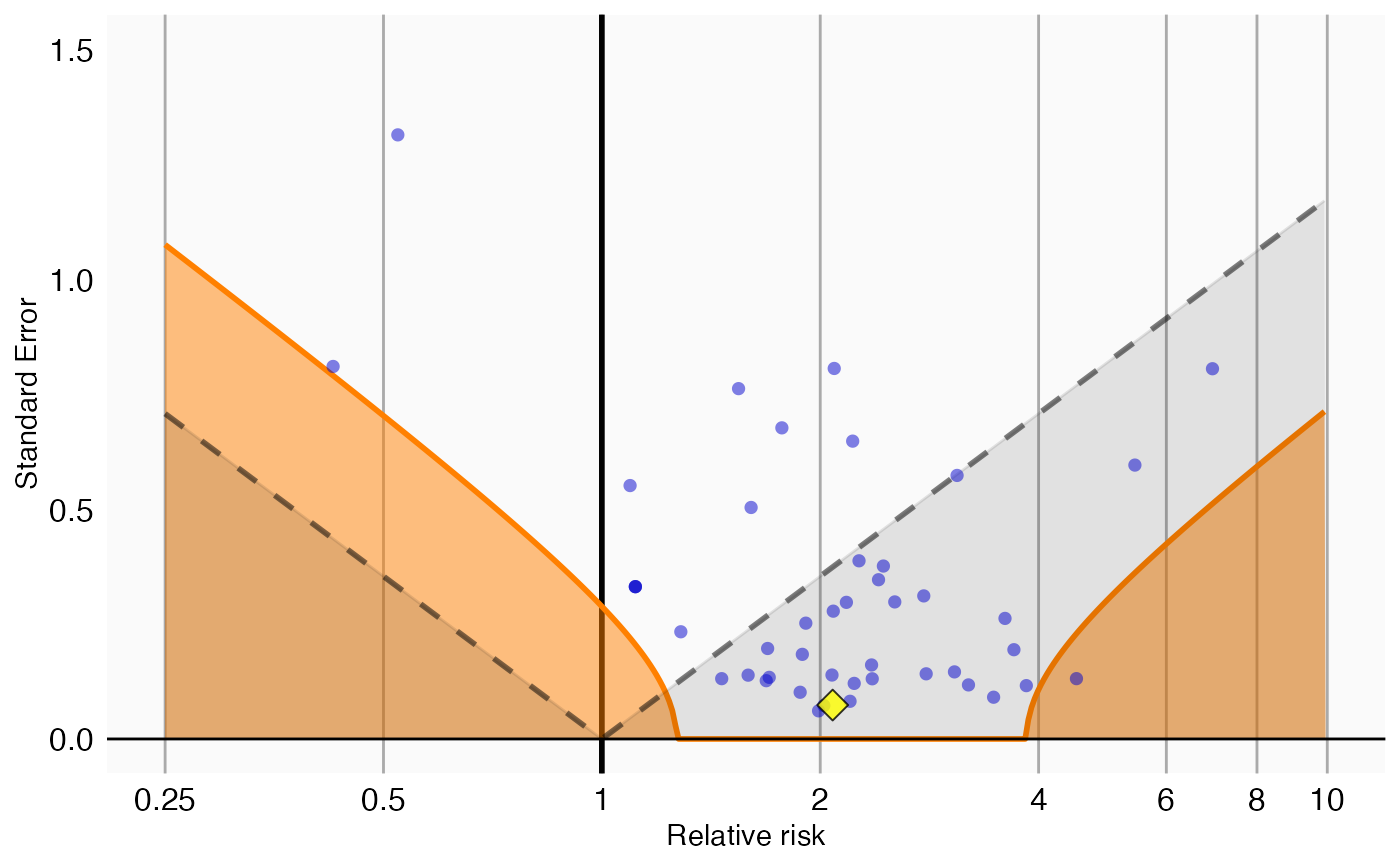
Creates a plot with the effect estimate on the x-axis and the standard error on the y-axis. Negative controls are shown as blue dots, positive controls as yellow diamonds. The area below the dashed line indicated estimates with p < 0.05. The orange area indicates estimates with calibrated p < 0.05.

Examples

data(sccs)
negatives <- sccs[sccs$groundTruth == 0, ]
positive <- sccs[sccs$groundTruth == 1, ]
plotCalibrationEffect(negatives$logRr, negatives$seLogRr, positive$logRr, positive$seLogRr)
#> Warning: Removed 1 rows containing missing values (`geom_vline()`).