Create a calibration plot

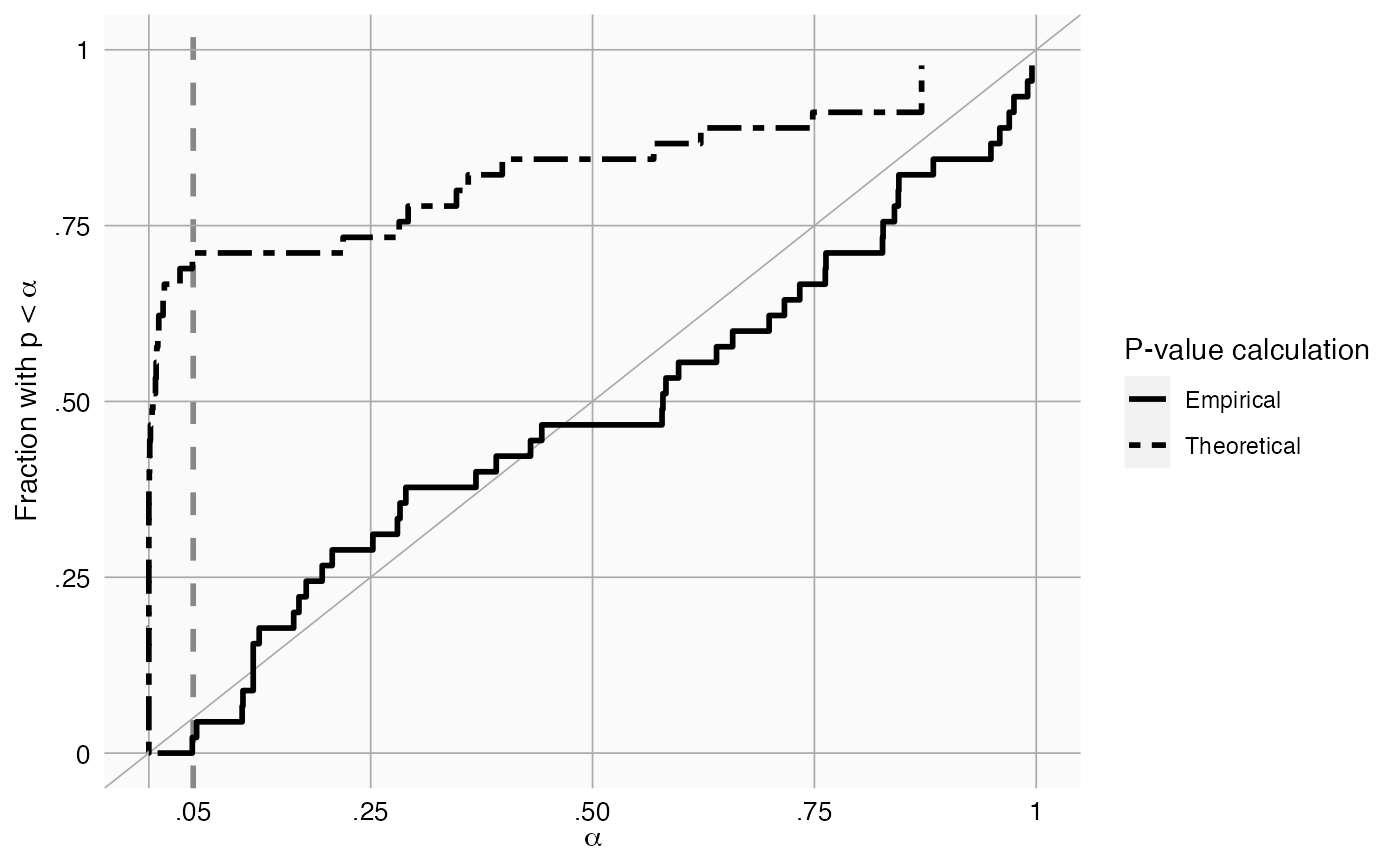
plotCalibration creates a plot showing the calibration of our calibration procedure

plotCalibration(
  logRr,
  seLogRr,
  useMcmc = FALSE,
  legendPosition = "right",
  title,
  fileName = NULL
)

Arguments

logRr

A numeric vector of effect estimates on the log scale

seLogRr

The standard error of the log of the effect estimates. Hint: often the standard error = (log(<lower bound 95 percent confidence interval>) - log(<effect estimate>))/qnorm(0.025)

useMcmc

Use MCMC to estimate the calibrated P-value?

legendPosition

Where should the legend be positioned? ("none", "left", "right", "bottom", "top")

title

Optional: the main title for the plot

fileName

Name of the file where the plot should be saved, for example 'plot.png'. See the function ggsave in the ggplot2 package for supported file formats.

Value

A Ggplot object. Use the ggsave function to save to file.

Details

Creates a calibration plot showing the number of effects with p < alpha for every level of alpha. The empirical calibration is performed using a leave-one-out design: The p-value of an effect is computed by fitting a null using all other negative controls. Ideally, the calibration line should approximate the diagonal. The plot shows both theoretical (traditional) and empirically calibrated p-values.

Examples

data(sccs)
negatives <- sccs[sccs$groundTruth == 0, ]
plotCalibration(negatives$logRr, negatives$seLogRr)