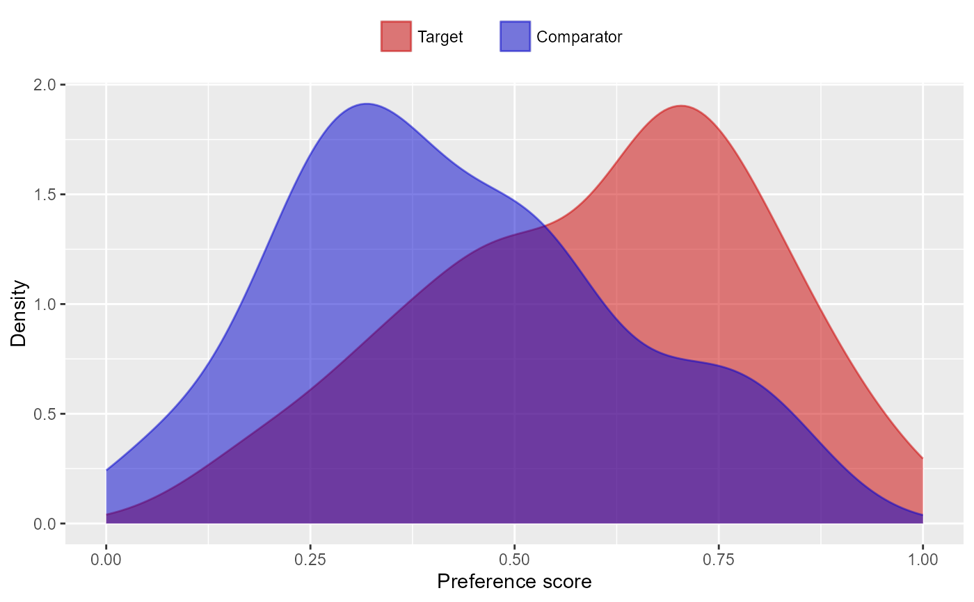
Plots the propensity (or preference) score distribution.
Usage
plotPs(
  data,
  unfilteredData = NULL,
  scale = "preference",
  type = "density",
  binWidth = 0.05,
  targetLabel = "Target",
  comparatorLabel = "Comparator",
  showCountsLabel = FALSE,
  showAucLabel = FALSE,
  showEquipoiseLabel = FALSE,
  equipoiseBounds = c(0.3, 0.7),
  unitOfAnalysis = "subjects",
  title = NULL,
  fileName = NULL
)
Arguments
- data
A data frame with at least the two columns described below
- unfilteredData
To be used when computing preference scores on data from which subjects have already been removed, e.g. through trimming and/or matching. This data frame should have the same structure as
data.- scale
The scale of the graph. Two scales are supported:
scale = 'propensity'orscale = 'preference'. The preference score scale is defined by Walker et al (2013).- type
Type of plot. Four possible values:
type = 'density'type = 'histogram',type = 'histogramCount', ortype = 'histogramProportion'.'histogram'defaults to'histogramCount'.- binWidth
For histograms, the width of the bins
- targetLabel
A label to us for the target cohort.
- comparatorLabel
A label to us for the comparator cohort.
- showCountsLabel
Show subject counts?
- showAucLabel
Show the AUC?
- showEquipoiseLabel
Show the percentage of the population in equipoise?
- equipoiseBounds
The bounds on the preference score to determine whether a subject is in equipoise.
- unitOfAnalysis
The unit of analysis in the input data. Defaults to 'subjects'.
- title
Optional: the main title for the plot.
- fileName
Name of the file where the plot should be saved, for example 'plot.png'. See the function
ggplot2::ggsave()for supported file formats.
Value
A ggplot object. Use the ggplot2::ggsave() function to save to file in a different
format.
Details
The data frame should have a least the following two columns:
treatment (integer): Column indicating whether the person is in the target (1) or comparator (0) group
propensityScore (numeric): Propensity score
References
Walker AM, Patrick AR, Lauer MS, Hornbrook MC, Marin MG, Platt R, Roger VL, Stang P, and Schneeweiss S. (2013) A tool for assessing the feasibility of comparative effectiveness research, Comparative Effective Research, 3, 11-20
Examples
treatment <- rep(0:1, each = 100)
propensityScore <- c(rnorm(100, mean = 0.4, sd = 0.25), rnorm(100, mean = 0.6, sd = 0.25))
data <- data.frame(treatment = treatment, propensityScore = propensityScore)
data <- data[data$propensityScore > 0 & data$propensityScore < 1, ]
plotPs(data)