Single studies using the CohortMethod package
Martijn J. Schuemie, Marc A. Suchard and Patrick Ryan
2026-06-19
Source:vignettes/SingleStudies.Rmd
SingleStudies.RmdIntroduction
This vignette describes how you can use the CohortMethod
package to perform a single new-user cohort study. We will walk through
all the steps needed to perform an exemplar study, and we have selected
the well-studied topic of the effect of coxibs versus non-selective
non-steroidal anti-inflammatory drugs (NSAIDs) on gastrointestinal (GI)
bleeding-related hospitalization. For simplicity, we focus on one coxib
– celecoxib – and one non-selective NSAID – diclofenac.
Data extraction
The first step in running the CohortMethod is extracting
all necessary data from the database server holding the data in the
Observational Medical Outcomes Partnership (OMOP) Common Data Model
(CDM) format.
Configuring the connection to the server
We need to tell R how to connect to the server where the data are.
CohortMethod uses the DatabaseConnector
package, which provides the createConnectionDetails
function. Type ?createConnectionDetails for the specific
settings required for the various database management systems (DBMS).
For example, one might connect to a PostgreSQL database using this
code:
library(CohortMethod)
connectionDetails <- createConnectionDetails(dbms = "postgresql",
                                             server = "localhost/ohdsi",
                                             user = "joe",
                                             password = "supersecret")

cdmDatabaseSchema <- "my_cdm_data"
cohortDatabaseSchema <- "my_results"
cohortTable <- "my_cohorts"
options(sqlRenderTempEmulationSchema = NULL)
The last few lines define the cdmDatabaseSchema,
cohortDatabaseSchema, and cohortTable
variables. We’ll use these later to tell R where the data in CDM format
live, and where we want to write intermediate tables. Note that for
Microsoft SQL Server, databaseschemas need to specify both the database
and the schema, so for example
cdmDatabaseSchema <- "my_cdm_data.dbo". For database
platforms that do not support temp tables, such as Oracle, it is also
necessary to provide a schema where the user has write access that can
be used to emulate temp tables. PostgreSQL supports temp tables, so we
can set options(sqlRenderTempEmulationSchema = NULL) (or
not set the sqlRenderTempEmulationSchema at all.)
Preparing the exposures and outcome(s)
We need to define the exposures and outcomes for our study. Here, we
will define our exposures using the OHDSI Capr package. We
define two exposure cohorts, one for celecoxib and one for diclofenac.
It is often a good idea to restrict your analysis to a specific
indication, to maximize the comparability of the two cohorts. In this
case, we will restrict to osteoarthritis of the knee. We will create a
cohort for this indication, starting a the first ever diagnosis, and
ending at observation period end.
library(Capr)

celecoxibConceptId <- 1118084
diclofenacConceptId <- 1124300
osteoArthritisOfKneeConceptId <- 4079750

celecoxib <- cs(
  descendants(celecoxibConceptId),
  name = "Celecoxib"
)

celecoxibCohort <- cohort(
  entry = entry(
    drugExposure(celecoxib)
  ),
  exit = exit(endStrategy = drugExit(celecoxib,
                                     persistenceWindow = 30,
                                     surveillanceWindow = 0))
)

diclofenac  <- cs(
  descendants(diclofenacConceptId),
  name = "Diclofenac"
)

diclofenacCohort <- cohort(
  entry = entry(
    drugExposure(diclofenac)
  ),
  exit = exit(endStrategy = drugExit(diclofenac,
                                     persistenceWindow = 30,
                                     surveillanceWindow = 0))
)

osteoArthritisOfKnee <- cs(
  descendants(osteoArthritisOfKneeConceptId),
  name = "Osteoarthritis of knee"
)

osteoArthritisOfKneeCohort <- cohort(
  entry = entry(
    conditionOccurrence(osteoArthritisOfKnee, firstOccurrence())
  ),
  exit = exit(
    endStrategy = observationExit()
  )
)
# Note: this will automatically assign cohort IDs 1,2, and 3, respectively:
exposuresAndIndicationCohorts <- makeCohortSet(celecoxibCohort,
                                               diclofenacCohort,
                                               osteoArthritisOfKneeCohort)
We’ll pull the outcome definition from the OHDSI
PhenotypeLibrary:
library(PhenotypeLibrary)
outcomeCohorts <- getPlCohortDefinitionSet(77) # GI bleed
We combine the exposure and outcome cohort definitions, and use
CohortGenerator to generate the cohorts:
allCohorts <- bind_rows(outcomeCohorts,
                        exposuresAndIndicationCohorts)

library(CohortGenerator)
cohortTableNames <- getCohortTableNames(cohortTable = cohortTable)
createCohortTables(connectionDetails = connectionDetails,
                   cohortDatabaseSchema = cohortDatabaseSchema,
                   cohortTableNames = cohortTableNames)
generateCohortSet(connectionDetails = connectionDetails,
                  cdmDatabaseSchema = cdmDatabaseSchema,
                  cohortDatabaseSchema = cohortDatabaseSchema,
                  cohortTableNames = cohortTableNames,
                  cohortDefinitionSet = allCohorts)
If all went well, we now have a table with the cohorts of interest. We can see how many entries per cohort:
connection <- DatabaseConnector::connect(connectionDetails)
sql <- "SELECT cohort_definition_id, COUNT(*) AS count
FROM @cohortDatabaseSchema.@cohortTable
GROUP BY cohort_definition_id"
cohortCounts <- DatabaseConnector::renderTranslateQuerySql(
  connection = connection,
  sql = sql,
  cohortDatabaseSchema = cohortDatabaseSchema,
  cohortTable = cohortTable
  )
DatabaseConnector::disconnect(connection)
## cohort_concept_id count
## 1 1 917230
## 2 2 1791695
## 3 3 993116
## 4 77 1123643Extracting the data from the server
Now we can tell CohortMethod to extract the cohorts,
construct covariates, and extract all necessary data for our
analysis.
Important: The target and comparator drug must not
be included in the covariates, including any descendant concepts. You
will need to manually add the drugs and descendants to the
excludedCovariateConceptIds of the covariate settings. In
this example code we exclude the concepts for celecoxib and diclofenac
and specify addDescendantsToExclude = TRUE:
# Define which types of covariates must be constructed:
covSettings <- createDefaultCovariateSettings(
  excludedCovariateConceptIds = c(diclofenacConceptId, celecoxibConceptId),
  addDescendantsToExclude = TRUE
)

#Load data:
cohortMethodData <- getDbCohortMethodData(
  connectionDetails = connectionDetails,
  cdmDatabaseSchema = cdmDatabaseSchema,
  targetId = 1,
  comparatorId = 2,
  outcomeIds = 77,
  exposureDatabaseSchema = cohortDatabaseSchema,
  exposureTable = cohortTable,
  outcomeDatabaseSchema = cohortDatabaseSchema,
  outcomeTable = cohortTable,
  nestingCohortDatabaseSchema = cohortDatabaseSchema,
  nestingCohortTable = cohortTable,
  getDbCohortMethodDataArgs = createGetDbCohortMethodDataArgs(
    removeDuplicateSubjects = "keep first, truncate to second",
    firstExposureOnly = TRUE,
    washoutPeriod = 365,
    restrictToCommonPeriod = TRUE,
    nestingCohortId = 3,
    covariateSettings = covSettings
  )
)
cohortMethodData
## # CovariateData object
##
## All cohorts
##
## Inherits from Andromeda:
## # Andromeda object
## # Physical location: C:\Users\admin_mschuemi.EU\AppData\Local\Temp\2\RtmpaKSoSG\file1fb833a136a9.duckdb
##
## Tables:
## $analysisRef (analysisId, analysisName, domainId, startDay, endDay, isBinary, missingMeansZero)
## $cohorts (rowId, personSeqId, personId, treatment, cohortStartDate, daysFromObsStart, daysToCohortEnd, daysToObsEnd)
## $covariateRef (covariateId, covariateName, analysisId, conceptId, valueAsConceptId, collisions)
## $covariates (rowId, covariateId, covariateValue)
## $outcomes (rowId, outcomeId, daysToEvent)There are many parameters, but they are all documented in the
CohortMethod manual. The
createDefaultCovariateSettings function is described in the
FeatureExtraction package. In short, we are pointing the
function to the table created earlier and indicating which concept IDs
in that table identify the target, comparator, nesting cohort and
outcome. We instruct that the default set of covariates should be
constructed, including covariates for all conditions, drug exposures,
and procedures that were found on or before the index date. To customize
the set of covariates, please refer to the
FeatureExtraction package vignette by typing
vignette("UsingFeatureExtraction", package="FeatureExtraction").
We let the CohortMethod package construct our sets of
new users: - For those patients who have exposure to both the target and
the comparator, we keep whichever is their first, and truncate their
exposure at the start of the second (if the first occurrences of the
target and comparator start simultaneously the patient is removed). - We
restrict to the first exposure overall (in this case redundant with the
previous step). - We require a washout period of 365 days, meaning any
patients with less than 365 days of prior observation are removed. - We
restrict to the period in time when both drugs were observed in the
database. This can be especially helpful when one of the exposures is
new to the market. - We restrict to the nesting cohort, in this case our
indication. Only exposures within the nesting cohort are kept.
We can see how many persons and exposures were left after each of these steps:
getAttritionTable(cohortMethodData)## description targetPersons comparatorPersons
## 1 Original cohorts 917230 993116
## 2 Keep first, truncate when e ... 845385 873667
## 3 First exposure only 845385 873667
## 4 365 days of prior observati ... 358646 515193
## 5 Restrict to common period 358646 515193
## 6 Restrict to nesting cohort 89318 128301
## targetExposures comparatorExposures
## 1 917230 993116
## 2 845385 873667
## 3 845385 873667
## 4 358646 515193
## 5 358646 515193
## 6 89318 128301The
cohortMethodData() function extracts all data about the exposures, outcomes, and covariates from the server and stores them in thecohortMethodDataobject. This object uses theAndromedapackage to store information in a way that ensures R does not run out of memory, even when the data are large. We can use the genericsummary()`
function to view some more information of the data we extracted:
summary(cohortMethodData)## Event count Person count
## 77 37448 20123Saving the data to file
Creating the cohortMethodData file can take considerable
computing time, and it is probably a good idea to save it for future
sessions. Because cohortMethodData uses
Andromeda, we cannot use R’s regular save function.
Instead, we’ll have to use the saveCohortMethodData()
function:
saveCohortMethodData(cohortMethodData, "coxibVsNonselVsGiBleed.zip")We can use the loadCohortMethodData() function to load
the data in a future session.
Defining the study population
Typically, the exposure cohorts and outcome cohorts will be defined
independently of each other. When we want to produce an effect size
estimate, we need to further restrict these cohorts and put them
together, for example by removing exposed subjects that had the outcome
prior to exposure, and only keeping outcomes that fall within a defined
risk window. For this we can use the createStudyPopulation
function:
studyPop <- createStudyPopulation(
  cohortMethodData = cohortMethodData,
  outcomeId = 77,
  createStudyPopulationArgs = createCreateStudyPopulationArgs(
    removeSubjectsWithPriorOutcome = TRUE,
    priorOutcomeLookback = 365,
    minDaysAtRisk = 1,
    riskWindowStart = 0,
    startAnchor = "cohort start",
    riskWindowEnd = 30,
    endAnchor = "cohort end"
  )
)
We specify the outcome ID we will use, and that people who had the
outcomes in the 365 days before the risk window start date will be
removed. The risk window is defined as starting at the cohort start date
(the index date, riskWindowStart = 0 and
startAnchor = "cohort start"), and the risk windows ends 30
days after the cohort ends (riskWindowEnd = 30 and
endAnchor = "cohort end"). Note that the risk windows are
truncated at the end of observation or the study end date. We also
remove subjects who have no time at risk. To see how many people are
left in the study population we can always use the
getAttritionTable function:
getAttritionTable(studyPop)## description targetPersons comparatorPersons
## 1 Original cohorts 917230 993116
## 2 Keep first, truncate when e ... 845385 873667
## 3 First exposure only 845385 873667
## 4 365 days of prior observati ... 358646 515193
## 5 Restrict to common period 358646 515193
## 6 Restrict to nesting cohort 89318 128301
## 7 No prior outcome 88134 126316
## 8 Have at least 1 days at ris ... 88134 126316
## targetExposures comparatorExposures
## 1 917230 993116
## 2 845385 873667
## 3 845385 873667
## 4 358646 515193
## 5 358646 515193
## 6 89318 128301
## 7 88134 126316
## 8 88134 126316Propensity scores
The CohortMethod can use propensity scores to adjust for
potential confounders. Instead of the traditional approach of using a
handful of predefined covariates, CohortMethod typically
uses tens of thousands of covariates that are automatically constructed
based on conditions, procedures and drugs in the records of the
subjects.
Fitting a propensity model
We can fit a propensity model using the covariates constructed by the
getDbcohortMethodData() function:
ps <- createPs(cohortMethodData = cohortMethodData, population = studyPop)The createPs() function uses the Cyclops
package to fit a large-scale regularized logistic regression.
To fit the propensity model, Cyclops needs to know the
hyperparameter value which specifies the variance of the prior. By
default Cyclops will use cross-validation to estimate the
optimal hyperparameter. However, be aware that this can take a really
long time. You can use the prior and control
parameters of the createPs() to specify
Cyclops behavior, including using multiple CPUs to speed-up
the cross-validation.
Propensity score diagnostics
We can compute the area under the receiver-operator curve (AUC) for the propensity score model:
computePsAuc(ps)## [1] 0.8411435We can also plot the propensity score distribution. By default, the
plotPS() function shows the preference score, a
transformation of the propensity score that adjusts for differences in
sizes between the target and comparator:
plotPs(ps,
       targetLabel = "Celexocib",
       comparatorLabel = "Diclofenac",
       showCountsLabel = TRUE,
       showAucLabel = TRUE,
       showEquipoiseLabel = TRUE)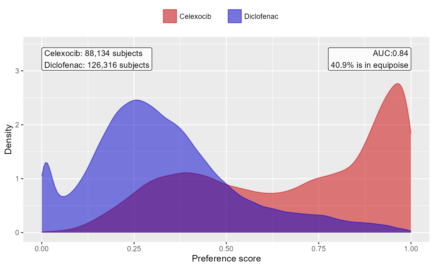
It is also possible to inspect the propensity model itself by showing the covariates that have non-zero coefficients:
getPsModel(ps, cohortMethodData)## # A tibble: 6 × 3
## coefficient covariateId covariateName
## <dbl> <dbl> <chr>
## 1 -4.11 1150871413 ...gh 0 days relative to index: misoprostol
## 2 3.26 2001006 index year: 2001
## 3 3.14 2002006 index year: 2002
## 4 2.67 2003006 index year: 2003
## 5 2.38 2004006 index year: 2004
## 6 1.67 2007006 index year: 2007One advantage of using the regularization when fitting the propensity model is that most coefficients will shrink to zero and fall out of the model. It is a good idea to inspect the remaining variables for anything that should not be there, for example variations of the drugs of interest that we forgot to exclude.
Finally, we can inspect the percent of the population in equipoise, meaning they have a preference score between 0.3 and 0.7:
CohortMethod::computeEquipoise(ps)## [1] 0.4090277A low equipoise indicates there is little overlap between the target and comparator populations.
Using the propensity score
We can use the propensity scores to trim, stratify, match, or weigh our population. For example, one could trim to equipoise, meaning only subjects with a preference score between 0.3 and 0.7 are kept:
trimmedPop <- trimByPs(ps,
                       trimByPsArgs = createTrimByPsArgs(
                         equipoiseBounds = c(0.3, 0.7)
                       ))
# Note: we need to also provide the original PS object so the preference score
# is computed using the original relative sizes of the cohorts:
plotPs(trimmedPop, ps)
## Trimming removed 55955 (63.5%) rows from the target, 70779 (56.0%) rows from the comparator in total.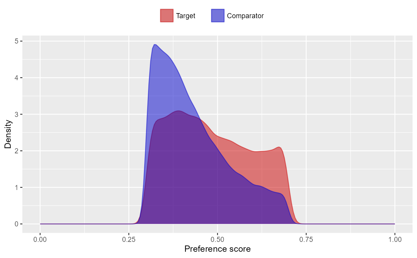
Instead (or additionally), we could stratify the population based on the propensity score:
stratifiedPop <- stratifyByPs(ps,
                              stratifyByPsArgs = createStratifyByPsArgs(
                                numberOfStrata = 5
                              ))
plotPs(stratifiedPop)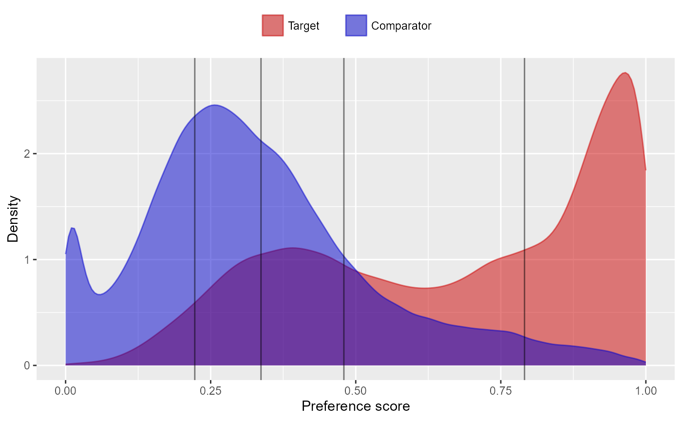
We can also match subjects based on propensity scores. In this
example, we’re using one-to-one matching. By default,
createPs() will use a caliper of 0.2 on the standardized
logit scale:
matchedPop <- matchOnPs(ps,
                        matchOnPsArgs = createMatchOnPsArgs(
                          maxRatio = 1
                        ))
plotPs(matchedPop, ps)
## Population size after matching is 96046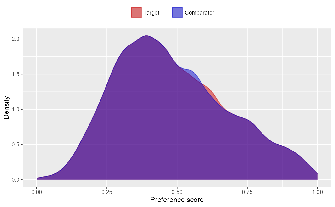
We can see the effect of trimming and/or matching on the population
using the getAttritionTable function:
getAttritionTable(matchedPop)## description targetPersons comparatorPersons
## 1 Original cohorts 917230 993116
## 2 Keep first, truncate when e ... 845385 873667
## 3 First exposure only 845385 873667
## 4 365 days of prior observati ... 358646 515193
## 5 Restrict to common period 358646 515193
## 6 Restrict to nesting cohort 89318 128301
## 7 Matched on propensity score 48023 48023
## targetExposures comparatorExposures
## 1 917230 993116
## 2 845385 873667
## 3 845385 873667
## 4 358646 515193
## 5 358646 515193
## 6 89318 128301
## 7 48023 48023Or, if we like, we can plot an attrition diagram:
drawAttritionDiagram(matchedPop)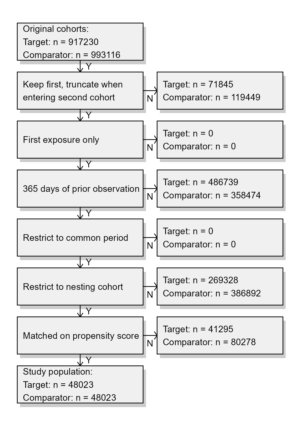
Evaluating covariate balance
To evaluate whether our use of the propensity score is indeed making the two cohorts more comparable, we can compute the covariate balance before and after trimming, matching, and/or stratifying:
balance <- computeCovariateBalance(matchedPop, cohortMethodData)
plotCovariateBalanceScatterPlot(balance,
                                showCovariateCountLabel = TRUE,
                                showMaxLabel = TRUE)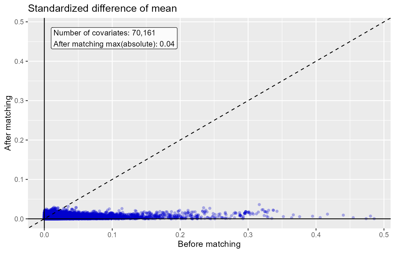
plotCovariateBalanceOfTopVariables(balance)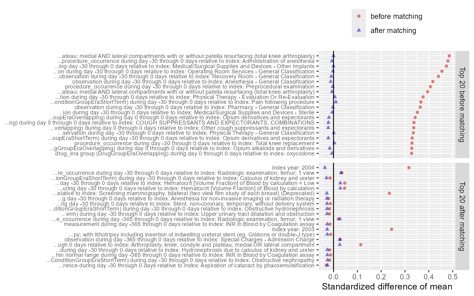
The ‘before matching’ population is the population as extracted by
the getDbCohortMethodData function, so before any further
filtering steps. We typically consider the populations to be balanced
if, after PS adjustment, all covariates have a standardized difference
of means smaller than 0.1.
Inspecting select population characteristics
It is customary to include a table in your paper that lists some
select population characteristics before and after
matching/stratification/trimming. This is usually the first table, and
so will be referred to as ‘table 1’. To generate this table, you can use
the createCmTable1 function:
createCmTable1(balance) Before matching After matching
Target Comparator Target Comparator
Characteristic % % Std. diff % % Std. diff
Age group
40 - 44 0.0 0.0 0.00 0.0 0.0 0.01
45 - 49 0.0 0.0 0.00 0.0 0.0 0.00
50 - 54 0.1 0.1 0.00 0.1 0.2 -0.01
55 - 59 0.4 0.5 -0.02 0.4 0.5 -0.01
60 - 64 0.9 1.3 -0.04 1.1 1.1 -0.01
65 - 69 22.9 21.2 0.04 22.5 22.4 0.00
70 - 74 28.3 26.6 0.04 27.3 27.2 0.00
75 - 79 22.0 20.9 0.03 21.3 21.5 -0.01
80 - 84 14.9 15.3 -0.01 15.2 15.1 0.00
85 - 89 7.4 9.3 -0.07 8.4 8.2 0.01
90 - 94 2.5 3.8 -0.07 3.0 3.0 0.00
95 - 99 0.5 0.9 -0.06 0.6 0.6 0.00
100 - 104 0.0 0.1 -0.02 0.1 0.1 0.00
105 - 109 0.0 0.0 -0.01 0.0 0.0 -0.01
Gender: female 62.9 67.2 -0.09 65.2 65.0 0.01
Medical history: General
Acute respiratory disease 21.7 25.4 -0.09 23.6 23.5 0.00
Attention deficit hyperactivity disorder 0.2 0.2 0.00 0.2 0.2 0.00
Chronic liver disease 1.0 1.5 -0.05 1.1 1.1 -0.01
Chronic obstructive pulmonary disease 9.6 11.3 -0.05 10.0 9.9 0.00
Crohn's disease 0.3 0.4 -0.02 0.4 0.4 0.00
Dementia 2.5 4.0 -0.08 3.0 2.9 0.00
Depressive disorder 9.1 11.9 -0.09 10.2 10.1 0.00
Diabetes mellitus 22.7 28.4 -0.13 24.7 24.6 0.00
Gastroesophageal reflux disease 16.1 19.4 -0.09 17.4 17.0 0.01
Gastrointestinal hemorrhage 3.5 3.8 -0.02 2.2 2.4 -0.01
Human immunodeficiency virus infection 0.0 0.1 -0.02 0.1 0.0 0.00
Hyperlipidemia 45.5 55.3 -0.20 49.6 48.6 0.02
Hypertensive disorder 63.2 69.7 -0.14 65.3 65.0 0.01
Lesion of liver 0.5 0.8 -0.04 0.5 0.5 0.00
Obesity 10.2 11.7 -0.05 10.0 9.7 0.01
Osteoarthritis 82.3 76.0 0.15 77.9 78.1 -0.01
Pneumonia 4.3 5.2 -0.05 4.3 4.3 0.00
Psoriasis 1.3 1.5 -0.02 1.4 1.3 0.01
Renal impairment 6.9 13.4 -0.22 8.3 8.1 0.01
Rheumatoid arthritis 3.1 3.9 -0.05 3.4 3.4 0.00
Schizophrenia 0.1 0.1 -0.01 0.1 0.1 0.00
Ulcerative colitis 0.5 0.6 -0.01 0.5 0.5 0.00
Urinary tract infectious disease 11.0 13.4 -0.08 11.8 11.8 0.00
Viral hepatitis C 0.2 0.3 -0.02 0.2 0.2 0.00
Medical history: Cardiovascular disease
Atrial fibrillation 9.8 11.8 -0.07 10.0 10.0 0.00
Cerebrovascular disease 11.2 12.8 -0.05 11.5 11.5 0.00
Coronary arteriosclerosis 19.2 20.9 -0.04 18.9 19.1 -0.01
Heart disease 43.4 44.8 -0.03 41.9 41.9 0.00
Heart failure 7.9 10.4 -0.08 7.8 7.9 0.00
Ischemic heart disease 9.1 9.6 -0.02 8.4 8.5 0.00
Peripheral vascular disease 8.8 12.5 -0.12 9.8 9.8 0.00
Pulmonary embolism 1.1 1.2 -0.02 1.1 1.1 0.00
Venous thrombosis 3.3 3.9 -0.03 3.4 3.6 -0.01
Medical history: Neoplasms
Malignant lymphoma 0.7 0.8 -0.01 0.8 0.8 0.00
Malignant neoplasm of anorectum 0.3 0.3 0.01 0.3 0.3 0.00
Malignant neoplastic disease 18.6 19.3 -0.02 19.0 19.1 0.00
Malignant tumor of breast 3.7 4.1 -0.02 3.9 3.9 0.00
Malignant tumor of colon 0.7 0.7 0.00 0.7 0.7 0.00
Malignant neoplasm of lung 0.3 0.4 -0.02 0.4 0.4 0.00
Malignant neoplasm of urinary bladder 0.9 0.8 0.00 0.9 0.8 0.01
Primary malignant neoplasm of prostate 3.8 3.3 0.02 3.6 3.6 0.00
Medication use
Agents acting on the renin-angiotensin system 50.1 53.4 -0.07 52.2 52.0 0.00
Antibacterials for systemic use 68.8 70.5 -0.04 68.6 68.6 0.00
Antidepressants 28.2 30.3 -0.05 30.0 30.1 0.00
Antiepileptics 20.0 21.6 -0.04 20.6 20.9 -0.01
Antiinflammatory and antirheumatic products 36.4 36.1 0.01 37.3 37.3 0.00
Antineoplastic agents 4.9 5.8 -0.04 5.2 5.1 0.00
Antipsoriatics 0.9 1.3 -0.05 0.9 1.0 -0.01
Antithrombotic agents 29.6 24.4 0.12 24.4 24.6 -0.01
Beta blocking agents 36.9 41.2 -0.09 38.3 38.0 0.01
Calcium channel blockers 28.1 31.4 -0.07 29.3 29.1 0.00
Diuretics 45.0 46.6 -0.03 45.2 45.4 0.00
Drugs for acid related disorders 41.1 43.1 -0.04 39.8 40.1 -0.01
Drugs for obstructive airway diseases 51.1 54.6 -0.07 53.6 53.0 0.01
Drugs used in diabetes 18.4 22.1 -0.09 19.6 19.5 0.00
Immunosuppressants 4.1 5.8 -0.08 4.8 4.6 0.01
Lipid modifying agents 55.2 59.2 -0.08 57.9 57.5 0.01
Opioids 64.7 55.1 0.20 58.5 59.0 -0.01
Psycholeptics 34.1 32.8 0.03 33.8 34.2 -0.01
Psychostimulants, agents used for adhd and nootropics 1.7 1.9 -0.02 2.0 2.1 -0.01 Generalizability
The goal of any propensity score adjustments is typically to make the
target and comparator cohorts comparably, to allow proper causal
inference. However, in doing so, we often need to modify our population,
for example dropping subjects that have no counterpart in the other
exposure cohort. The population we end up estimating an effect for may
end up being very different from the population we started with. An
important question is: how different? And it what ways? If the
populations before and after adjustment are very different, our
estimated effect may not generalize to the original population (if
effect modification is present). The
getGeneralizabilityTable() function informs on these
differences:
getGeneralizabilityTable(balance)
[38;5;246m# A tibble: 85,838 × 5
[39m
   covariateId covariateName        beforeMatchingMean afterMatchingMean stdDiff

[3m
[38;5;246m<dbl>
[39m
[23m
[3m
[38;5;246m<chr>
[39m
[23m
[3m
[38;5;246m<dbl>
[39m
[23m
[3m
[38;5;246m<dbl>
[39m
[23m
[3m
[38;5;246m<dbl>
[39m
[23m

[38;5;250m 1
[39m
[4m4
[24m160
[4m4
[24m
[4m3
[24m
[4m9
[24m504 ...: Administration…             0.157             0.029
[4m9
[24m   0.447

[38;5;250m 2
[39m
[4m2
[24m105
[4m1
[24m
[4m0
[24m
[4m3
[24m504 ...cing (total knee…             0.116             0.010
[4m2
[24m   0.446

[38;5;250m 3
[39m
[4m3
[24m
[4m8
[24m003
[4m1
[24m
[4m6
[24m
[4m2
[24m804 ...s and Devices - …             0.124             0.018
[4m5
[24m   0.420

[38;5;250m 4
[39m
[4m3
[24m
[4m8
[24m003
[4m2
[24m
[4m0
[24m
[4m8
[24m804 ...vices - General …             0.139             0.029
[4m6
[24m   0.401

[38;5;250m 5
[39m
[4m3
[24m
[4m8
[24m003
[4m3
[24m
[4m9
[24m
[4m0
[24m804 ... Room - General …             0.132             0.027
[4m9
[24m   0.391

[38;5;250m 6
[39m
[4m3
[24m
[4m8
[24m003
[4m2
[24m
[4m1
[24m
[4m3
[24m804 ...hesia - General …             0.120             0.024
[4m7
[24m   0.374

[38;5;250m 7
[39m   764
[4m6
[24m
[4m0
[24m
[4m8
[24m504 ...dex: Preprocedur…             0.097
[4m8
[24m            0.015
[4m6
[24m   0.361

[38;5;250m 8
[39m
[4m3
[24m
[4m8
[24m003
[4m2
[24m
[4m4
[24m
[4m5
[24m804 ... - Evaluation Or…             0.118             0.030
[4m2
[24m   0.339

[38;5;250m 9
[39m
[4m3
[24m
[4m8
[24m003
[4m1
[24m
[4m3
[24m
[4m8
[24m804 ...rmacy - General …             0.175             0.069
[4m2
[24m   0.326

[38;5;250m10
[39m
[4m4
[24m002
[4m0
[24m
[4m1
[24m
[4m4
[24m212 ...ndex: Pain follo…             0.075
[4m3
[24m            0.011
[4m0
[24m   0.321

[38;5;246m# ℹ 85,828 more rows
[39m
In this case, because we used PS matching, we are likely aiming to
estimate the average treatment effect in the treated (ATT). For this
reason, the getGeneralizabilityTable() function
automatically selected the target cohort as the basis for evaluating
generalizability: it shows, for each covariate, the mean value before
and PS adjustment in the target cohort. Also shown is the standardized
difference of mean, and the table is reverse sorted by the absolute
standard difference of mean (ASDM).
Follow-up and power
Before we start fitting an outcome model, we might be interested to know whether we have sufficient power to detect a particular effect size. It makes sense to perform these power calculations once the study population has been fully defined, so taking into account loss to the various inclusion and exclusion criteria (such as no prior outcomes), and loss due to matching and/or trimming. Since the sample size is fixed in retrospective studies (the data has already been collected), and the true effect size is unknown, the CohortMethod package provides a function to compute the minimum detectable relative risk (MDRR) instead:
computeMdrr(
  population = studyPop,
  modelType = "cox",
  alpha = 0.05,
  power = 0.8,
  twoSided = TRUE
)
## targetPersons comparatorPersons targetExposures comparatorExposures
## 1 88134 126316 88134 126316
## targetDays comparatorDays totalOutcomes mdrr se
## 1 12087401 9619724 1252 1.174598 0.05744113In this example we used the studyPop object, so the
population before any matching or trimming. If we want to know the MDRR
after matching, we use the matchedPop object we created
earlier instead:
computeMdrr(
  population = matchedPop,
  modelType = "cox",
  alpha = 0.05,
  power = 0.8,
  twoSided = TRUE
)
## targetPersons comparatorPersons targetExposures comparatorExposures
## 1 48023 48023 48023 48023
## targetDays comparatorDays totalOutcomes mdrr se
## 1 6752916 3896834 597 1.257748 0.08185455Even thought the MDRR in the matched population is higher, meaning we have less power, we should of course not be fooled: matching most likely eliminates confounding, and is therefore preferred to not matching.
To gain a better understanding of the amount of follow-up available
we can also inspect the distribution of follow-up time. We defined
follow-up time as time at risk, so not censored by the occurrence of the
outcome. The getFollowUpDistribution can provide a simple
overview:
getFollowUpDistribution(population = matchedPop)## 100% 75% 50% 25% 0% Treatment
## 1 1 60 60 130 3486 1
## 2 1 45 60 71 3833 0The output is telling us number of days of follow-up each quantile of the study population has. We can also plot the distribution:
plotFollowUpDistribution(population = matchedPop)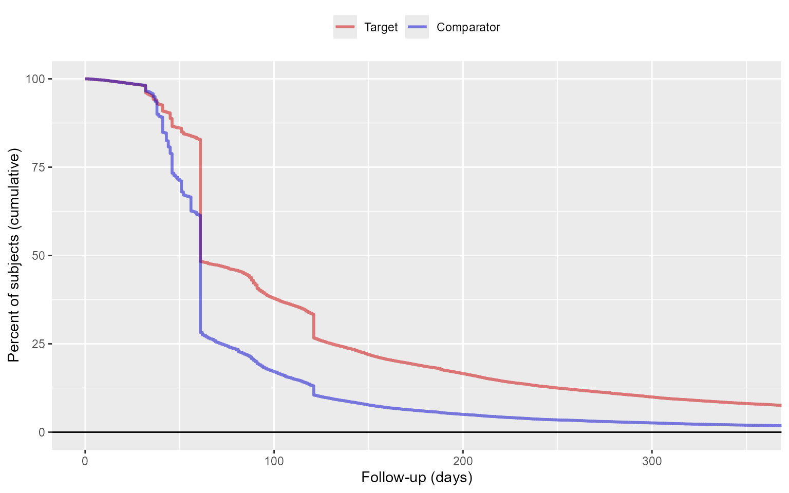
Outcome models
The outcome model is a model describing which variables are associated with the outcome.
Fitting a simple outcome model
In theory we could fit an outcome model without using the propensity scores. In this example we are fitting an outcome model using a Cox regression:
outcomeModel <- fitOutcomeModel(
  population = studyPop,
  fitOutcomeModelArgs = createFitOutcomeModelArgs(
    modelType = "cox"
  )
)
outcomeModel
## Estimate lower .95 upper .95 logRr seLogRr
## treatment 0.961778 0.856018 1.080701 -0.038971 0.0595But of course we want to make use of the matching done on the propensity score:
outcomeModel <- fitOutcomeModel(
  population = matchedPop,
  fitOutcomeModelArgs = createFitOutcomeModelArgs(
    modelType = "cox"
  )
)
outcomeModel
## Estimate lower .95 upper .95 logRr seLogRr
## treatment 0.84469 0.71412 1.00030 -0.16878 0.086Note that we define the sub-population to be only those in the
matchedPop object, which we created earlier by matching on
the propensity score.
Instead of matching or stratifying we can also perform Inverse Probability of Treatment Weighting (IPTW):
outcomeModel <- fitOutcomeModel(
  population = ps,
  fitOutcomeModelArgs = createFitOutcomeModelArgs(
    modelType = "cox",
    inversePtWeighting = TRUE,
    bootstrapCi = TRUE
  )
)
outcomeModel
## Estimate lower .95 upper .95 logRr seLogRr
## treatment 0.66899 0.47331 0.97783 -0.40199 0.178Note that in this case we may want to use a bootstrap to compute the confidence interval.
Adding interaction terms
We may be interested whether the effect is different across different groups in the population. To explore this, we may include interaction terms in the model. In this example we include three interaction terms:
interactionCovariateIds <- c(8532001, 201826210, 21600960413)
# 8532001 = Female
# 201826210 = Type 2 Diabetes
# 21600960413 = Concurent use of antithrombotic agents
outcomeModel <- fitOutcomeModel(
  population = matchedPop,
  cohortMethodData = cohortMethodData,
  fitOutcomeModelArgs = createFitOutcomeModelArgs(
    modelType = "cox",
    interactionCovariateIds = interactionCovariateIds
  )
)
outcomeModel
## Estimate
## treatment 0.809658
## treatment * condition_era group (ConditionGroupEraLongTerm) during day -365 through 0 days relative to index: Type 2 diabetes mellitus 0.860438
## treatment * drug_era group (DrugGroupEraOverlapping) during day 0 through 0 days relative to index: ANTITHROMBOTIC AGENTS 1.011228
## treatment * gender = FEMALE 1.111761
## lower .95
## treatment 0.590267
## treatment * condition_era group (ConditionGroupEraLongTerm) during day -365 through 0 days relative to index: Type 2 diabetes mellitus 0.601425
## treatment * drug_era group (DrugGroupEraOverlapping) during day 0 through 0 days relative to index: ANTITHROMBOTIC AGENTS 0.701484
## treatment * gender = FEMALE 0.791320
## upper .95
## treatment 1.113710
## treatment * condition_era group (ConditionGroupEraLongTerm) during day -365 through 0 days relative to index: Type 2 diabetes mellitus 1.233185
## treatment * drug_era group (DrugGroupEraOverlapping) during day 0 through 0 days relative to index: ANTITHROMBOTIC AGENTS 1.462634
## treatment * gender = FEMALE 1.560599
## logRr
## treatment -0.211144
## treatment * condition_era group (ConditionGroupEraLongTerm) during day -365 through 0 days relative to index: Type 2 diabetes mellitus -0.150314
## treatment * drug_era group (DrugGroupEraOverlapping) during day 0 through 0 days relative to index: ANTITHROMBOTIC AGENTS 0.011166
## treatment * gender = FEMALE 0.105946
## seLogRr
## treatment 0.1620
## treatment * condition_era group (ConditionGroupEraLongTerm) during day -365 through 0 days relative to index: Type 2 diabetes mellitus 0.1832
## treatment * drug_era group (DrugGroupEraOverlapping) during day 0 through 0 days relative to index: ANTITHROMBOTIC AGENTS 0.1875
## treatment * gender = FEMALE 0.1732It is prudent to verify that covariate balance has also been achieved in the subgroups of interest. For example, we can check the covariate balance in the subpopulation of females:
balanceFemale <- computeCovariateBalance(
  population,
  cohortMethodData,
  computeCovariateBalanceArgs = createComputeCovariateBalanceArgs(
    subgroupCovariateId = 8532001
  )
)
plotCovariateBalanceScatterPlot(balanceFemale)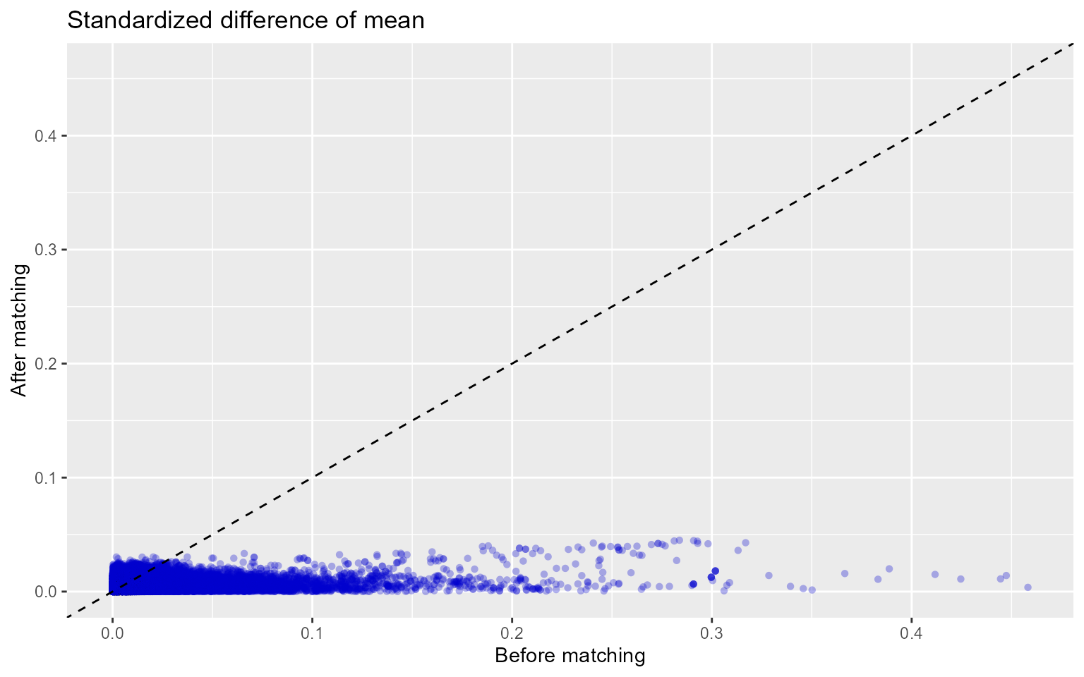
Adding covariates to the outcome model
One final refinement would be to use the same covariates we used to
fit the propensity model to also fit the outcome model. This way we are
more robust against misspecification of the model, and more likely to
remove bias. For this we use the regularized Cox regression in the
Cyclops package. (Note that the treatment variable is
automatically excluded from regularization.)
outcomeModel <- fitOutcomeModel(
  population = matchedPop,
  cohortMethodData = cohortMethodData,
  fitOutcomeModelArgs = createFitOutcomeModelArgs(
    modelType = "cox",
    useCovariates = TRUE,
  )
)
outcomeModel
## Estimate lower .95 upper .95 logRr seLogRr
## treatment 0.925449 0.717305 1.194886 -0.077476 0.1302Inspecting the outcome model
We can inspect more details of the outcome model:
## 4393168283078717
## 0.9254494## [1] 0.7173049 1.1948858We can also see the covariates that ended up in the outcome model:
getOutcomeModel(outcomeModel, cohortMethodData)## coefficient id name
## 1 -0.0774758 4.393168e+15 TreatmentKaplan-Meier plot
We can create the Kaplan-Meier plot:
plotKaplanMeier(matchedPop, includeZero = FALSE)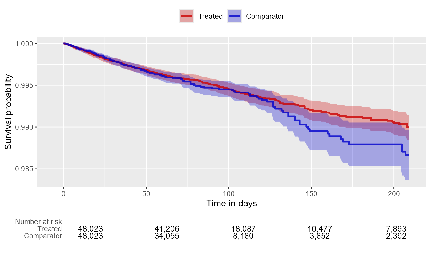
Note that the Kaplan-Meier plot will automatically adjust for any stratification, matching, or trimming that may have been applied.
Time-to-event plot
We can also plot time-to-event, showing both events before and after the index date, and events during and outside the defined time-at-risk window. This plot can provide insight into the temporal pattern of the outcome relative to the exposures:
plotTimeToEvent(
  cohortMethodData = cohortMethodData,
  outcomeId = 77,
  minDaysAtRisk = 1,
  riskWindowStart = 0,
  startAnchor = "cohort start",
  riskWindowEnd = 30,
  endAnchor = "cohort end"
)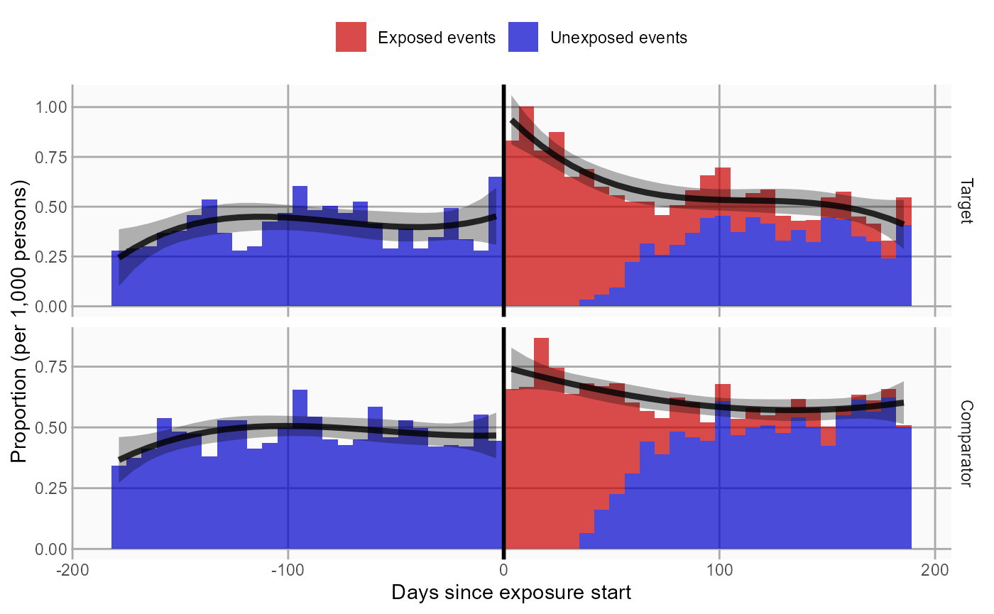
Note that this plot does not show any adjustment for the propensity score.
Acknowledgments
Considerable work has been dedicated to provide the
CohortMethod package.
citation("CohortMethod")## To cite CohortMethod in publications use:
##
## Schuemie MJ, Reps JM, Black A, DeFalco F, Evans L, Fridgeirsson E,
## Gilbert JP, Knoll C, Lavallee M, Rao G, Rijnbeek P, Sadowski K, Sena
## A, Swerdel J, Williams RD, Suchard MA (2024). "Health-analytics data
## to evidence suite (HADES): open-source software for observational
## research." _Studies in Health Technology and Informatics_, *310*,
## 966-970. doi:10.3233/SHTI231108 <https://doi.org/10.3233/SHTI231108>,
## <https://doi.org/10.3233/shti231108>.
##
## A BibTeX entry for LaTeX users is
##
## @Article{,
## title = {Health-analytics data to evidence suite (HADES): open-source software for observational research},
## author = {M. J. Schuemie and J. M. Reps and A. Black and F. DeFalco and L. Evans and E. Fridgeirsson and J. P. Gilbert and C. Knoll and M. Lavallee and G. Rao and P. Rijnbeek and K. Sadowski and A. Sena and J. Swerdel and R. D. Williams and M. A. Suchard},
## journal = {Studies in Health Technology and Informatics},
## year = {2024},
## volume = {310},
## pages = {966-970},
## doi = {10.3233/SHTI231108},
## url = {https://doi.org/10.3233/shti231108},
## }Further, CohortMethod makes extensive use of the
Cyclops package.
citation("Cyclops")## To cite Cyclops in publications use:
##
## Suchard MA, Simpson SE, Zorych I, Ryan P, Madigan D (2013). "Massive
## parallelization of serial inference algorithms for complex
## generalized linear models." _ACM Transactions on Modeling and
## Computer Simulation_, *23*, 10. doi:10.1145/2414416.2414791
## <https://doi.org/10.1145/2414416.2414791>.
##
## A BibTeX entry for LaTeX users is
##
## @Article{,
## author = {M. A. Suchard and S. E. Simpson and I. Zorych and P. Ryan and D. Madigan},
## title = {Massive parallelization of serial inference algorithms for complex generalized linear models},
## journal = {ACM Transactions on Modeling and Computer Simulation},
## volume = {23},
## pages = {10},
## year = {2013},
## doi = {10.1145/2414416.2414791},
## }This work is supported in part through the National Science Foundation grant IIS 1251151.