Running multiple analyses at once using the CohortMethod package
Martijn J. Schuemie, Marc A. Suchard and Patrick Ryan
2026-06-19
Source:vignettes/MultipleAnalyses.Rmd
MultipleAnalyses.RmdIntroduction
In this vignette we focus on running several different analyses on several target-comparator-(nesting)- outcome combinations. This can be useful when we want to explore the sensitivity to analyses choices, include controls, or run an experiment similar to the OMOP experiment to empirically identify the optimal analysis choices for a particular research question.
This vignette assumes you are already familiar with the
CohortMethod package and are able to perform single
studies. We will walk through all the steps needed to perform an
exemplar set of analyses, and we have selected the well-studied topic of
the effect of coxibs versus non-selective nonsteroidal anti-inflammatory
drugs (NSAIDs) on gastrointestinal (GI) bleeding-related
hospitalization. For simplicity, we focus on one coxib – celecoxib – and
one non-selective NSAID – diclofenac. We will execute various variations
of an analysis for the primary outcome and a large set of negative
control outcomes.
General approach
The general approach to running a set of analyses is that you specify all the function arguments of the functions you would normally call, and create sets of these function arguments. The final outcome models as well as intermediate data objects will all be saved to disk for later extraction.
An analysis will be executed by calling these functions in sequence:
getDbCohortMethodData()createStudyPopulation()-
createPs()(optional) -
trimByPs()(optional) -
matchOnPs()orstratifyByPs()(optional) -
computeCovariateBalance()(optional) -
fitOutcomeModel()(optional)
When you provide several analyses to the CohortMethod
package, it will determine whether any of the analyses have anything in
common, and will take advantage of this fact. For example, if we specify
several analyses that only differ in the way the outcome model is
fitted, then CohortMethod will extract the data and fit the
propensity model only once, and re-use this in all the analyses.
The function arguments you need to define have been divided into four groups:
- Hypothesis of interest: arguments that are specific to a hypothesis of interest, in the case of the cohort method this is a combination of target, comparator, nesting cohort (optional) and outcome.
- Analyses: arguments that are not directly specific to a hypothesis of interest, such as the washout window, whether to include drugs as covariates, etc.
- Arguments that are the output of a previous function in the
CohortMethodpackage, such as thecohortMethodDataargument of thecreatePsfunction. These cannot be specified by the user. - Arguments that are specific to an environment, such as the connection details for connecting to the server, and the name of the schema holding the CDM data.
There are a two arguments (excludedCovariateConceptIds,
and includedCovariateConceptIds of the
covariateSettings argument of
getDbCohortMethodData()) that can be argued to be part both
of group 1 and 2. These arguments are therefore present in both groups,
and when executing the analysis the union of the two lists of concept
IDs will be used.
Preparation for the example
We need to tell R how to connect to the server where the data are.
CohortMethod uses the DatabaseConnector
package, which provides the createConnectionDetails
function. Type ?createConnectionDetails for the specific
settings required for the various database management systems (DBMS).
For example, one might connect to a PostgreSQL database using this
code:
connectionDetails <- createConnectionDetails(dbms = "postgresql",
                                             server = "localhost/ohdsi",
                                             user = "joe",
                                             password = "supersecret")

cdmDatabaseSchema <- "my_cdm_data"
cohortDatabaseSchema <- "my_results"
cohortTable <- "my_cohorts"
options(sqlRenderTempEmulationSchema = NULL)
The last few lines define the cdmDatabaseSchema,
cohortDatabaseSchema, and cohortTable
variables. We’ll use these later to tell R where the data in CDM format
live, and where we want to write intermediate tables. Note that for
Microsoft SQL Server, databaseschemas need to specify both the database
and the schema, so for example
cdmDatabaseSchema <- "my_cdm_data.dbo". For database
platforms that do not support temp tables, such as Oracle, it is also
necessary to provide a schema where the user has write access that can
be used to emulate temp tables. PostgreSQL supports temp tables, so we
can set options(sqlRenderTempEmulationSchema = NULL) (or
not set the sqlRenderTempEmulationSchema at all.)
Preparing the exposures and outcome(s)
We need to define the exposures and outcomes for our study. Here, we
will define our exposures using the OHDSI Capr package. We
define two exposure cohorts, one for celecoxib and one for diclofenac.
It is often a good idea to restrict your analysis to a specific
indication, to maximize the comparability of the two cohorts. In this
case, we will restrict to osteoarthritis of the knee. We will create a
cohort for this indication, starting a the first ever diagnosis, and
ending at observation period end.
library(Capr)

celecoxibConceptId <- 1118084
diclofenacConceptId <- 1124300
osteoArthritisOfKneeConceptId <- 4079750

celecoxib <- cs(
  descendants(celecoxibConceptId),
  name = "Celecoxib"
)

celecoxibCohort <- cohort(
  entry = entry(
    drugExposure(celecoxib)
  ),
  exit = exit(endStrategy = drugExit(celecoxib,
                                     persistenceWindow = 30,
                                     surveillanceWindow = 0))
)

diclofenac  <- cs(
  descendants(diclofenacConceptId),
  name = "Diclofenac"
)

diclofenacCohort <- cohort(
  entry = entry(
    drugExposure(diclofenac)
  ),
  exit = exit(endStrategy = drugExit(diclofenac,
                                     persistenceWindow = 30,
                                     surveillanceWindow = 0))
)

osteoArthritisOfKnee <- cs(
  descendants(osteoArthritisOfKneeConceptId),
  name = "Osteoarthritis of knee"
)

osteoArthritisOfKneeCohort <- cohort(
  entry = entry(
    conditionOccurrence(osteoArthritisOfKnee, firstOccurrence())
  ),
  exit = exit(
    endStrategy = observationExit()
  )
)
# Note: this will automatically assign cohort IDs 1,2, and 3, respectively:
exposuresAndIndicationCohorts <- makeCohortSet(celecoxibCohort,
                                               diclofenacCohort,
                                               osteoArthritisOfKneeCohort)
We’ll pull the outcome definition from the OHDSI
PhenotypeLibrary:
library(PhenotypeLibrary)
outcomeCohorts <- getPlCohortDefinitionSet(77) # GI bleed
In addition to the outcome of interest, we also want to include a large set of negative control outcomes. For simplicity we define each negative control as a concept and all of its descendants:
negativeControlIds <- c(29735, 140673, 197494,
                        198185, 198199, 200528, 257315,
                        314658, 317376, 321319, 380731,
                        432661, 432867, 433516, 433701,
                        433753, 435140, 435459, 435524,
                        435783, 436665, 436676, 442619,
                        444252, 444429, 4131756, 4134120,
                        4134454, 4152280, 4165112, 4174262,
                        4182210, 4270490, 4286201, 4289933)
negativeControlCohorts <- tibble(
  cohortId = negativeControlIds,
  cohortName = sprintf("Negative control %d", negativeControlIds),
  outcomeConceptId = negativeControlIds
)
We combine the exposure, indication and outcome cohort definitions,
and use CohortGenerator to generate the cohorts:
library(CohortGenerator)
allCohorts <- bind_rows(outcomeCohorts,
                        exposuresAndIndicationCohorts)
cohortTableNames <- getCohortTableNames(cohortTable = cohortTable)
createCohortTables(connectionDetails = connectionDetails,
                   cohortDatabaseSchema = cohortDatabaseSchema,
                   cohortTableNames = cohortTableNames)
generateCohortSet(connectionDetails = connectionDetails,
                  cdmDatabaseSchema = cdmDatabaseSchema,
                  cohortDatabaseSchema = cohortDatabaseSchema,
                  cohortTableNames = cohortTableNames,
                  cohortDefinitionSet = allCohorts)
generateNegativeControlOutcomeCohorts(connectionDetails = connectionDetails,
                                      cdmDatabaseSchema = cdmDatabaseSchema,
                                      cohortDatabaseSchema = cohortDatabaseSchema,
                                      cohortTableNames  = cohortTableNames,
                                      negativeControlOutcomeCohortSet = negativeControlCohorts)
If all went well, we now have a table with the cohorts of interest. We can see how many entries per cohort:
connection <- DatabaseConnector::connect(connectionDetails)
sql <- "SELECT cohort_definition_id, COUNT(*) AS count
FROM @cohortDatabaseSchema.@cohortTable
GROUP BY cohort_definition_id"
DatabaseConnector::renderTranslateQuerySql(
  connection = connection,
  sql = sql,
  cohortDatabaseSchema = cohortDatabaseSchema,
  cohortTable = cohortTable
  )
DatabaseConnector::disconnect(connection)
## cohort_definition_id count
## 1 4182210 4430749
## 2 4134120 51817
## 3 4152280 2125215
## 4 257315 982236
## 5 317376 74848
## 6 314658 3305406
## 7 4174262 1332706
## 8 4286201 216303
## 9 4134454 17972
## 10 433701 90997
## 11 435783 178528
## 12 140673 8957971
## 13 380731 106693
## 14 433516 236503
## 15 197494 114327
## 16 432867 37075900
## 17 198199 215692
## 18 436665 717207
## 19 436676 431672
## 20 200528 979211
## 21 444429 170621
## 22 433753 496482
## 23 435524 356849
## 24 442619 1036
## 25 435459 155207
## 26 29735 324877
## 27 432661 990
## 28 3 1791695
## 29 2 993116
## 30 321319 1337722
## 31 1 917230
## 32 77 1123643Specifying hypotheses of interest
The first group of arguments define the target, comparator, nesting(optional), and outcome. Here we demonstrate how to create one set, and add that set to a list:
outcomeOfInterest <- createOutcome(outcomeId = 77,
                                   outcomeOfInterest = TRUE)
negativeControlOutcomes <- lapply(
  negativeControlIds,
  function(outcomeId) createOutcome(outcomeId = outcomeId,
                                    outcomeOfInterest = FALSE,
                                    trueEffectSize = 1)
)
tcos <- createTargetComparatorOutcomes(
  targetId = 1,
  comparatorId = 2,
  nestingCohortId = 3,
  outcomes = append(list(outcomeOfInterest),
                    negativeControlOutcomes),
  excludedCovariateConceptIds = c(1118084, 1124300)
)
targetComparatorOutcomesList <- list(tcos)
We first define the outcome of interest (GI-bleed, cohort ID 77),
explicitly stating this is an outcome of interest
(outcomeOfInterest = TRUE), meaning we want the full set of
artifacts generated for this outcome. We then create a set of negative
control outcomes. Because we specify
outcomeOfInterest = FALSE, many of the artifacts will not
be saved (like the matched population), or even not generated at all
(like the covariate balance). This can save a lot of compute time and
disk space. We also provide the true effect size for these controls,
which will be used later for empirical calibration. We set the target to
be celecoxib (cohort ID 1), the comparator to be diclofenac (cohort ID
2), and the nesting cohort to osteoarthritis of the knee (cohort ID
3).
A convenient way to save targetComparatorOutcomesList to
file is by using the saveTargetComparatorOutcomesList
function, and we can load it again using the
loadTargetComparatorOutcomesList function.
Specifying analyses
The second group of arguments are not specific to a hypothesis of
interest, and comprise the majority of arguments. You can recognize
these arguments because they are created by a separate ‘create…Args’
function. For example, for the gtDbCohortMethodData()
function there is the createGetDbCohortMethodDataArgs()
function. These settings functions can be used to create the arguments
to be used during execution:
covarSettings <- createDefaultCovariateSettings(
  addDescendantsToExclude = TRUE
)

getDbCmDataArgs <- createGetDbCohortMethodDataArgs(
  removeDuplicateSubjects = "keep first, truncate to second",
  firstExposureOnly = TRUE,
  washoutPeriod = 183,
  restrictToCommonPeriod = TRUE,
  covariateSettings = covarSettings
)

createStudyPopArgs <- createCreateStudyPopulationArgs(
  removeSubjectsWithPriorOutcome = TRUE,
  minDaysAtRisk = 1,
  riskWindowStart = 0,
  startAnchor = "cohort start",
  riskWindowEnd = 30,
  endAnchor = "cohort end"
)

fitOutcomeModelArgs1 <- createFitOutcomeModelArgs(
  modelType = "cox"
)
Note that, when calling
createDefaultCovariateSettings(), we do not specify the
covariates to exclude. When running the analysis,
CohortMethod will automatically add the
excludedCovariateConceptIds specified earlier when calling
createTargetComparatorOutcomes(). This allows the same
analyses settings to be used for multiple TCOs.
Any argument that is not explicitly specified by the user will assume the default value specified in the function. We can now combine the arguments for the various functions into a single analysis:
cmAnalysis1 <- createCmAnalysis(
  analysisId = 1,
  description = "No matching, simple outcome model",
  getDbCohortMethodDataArgs = getDbCmDataArgs,
  createStudyPopulationArgs = createStudyPopArgs,
  fitOutcomeModelArgs = fitOutcomeModelArgs1
)
Note that we have assigned an analysis ID (1) to this set of arguments. We can use this later to link the results back to this specific set of choices. We also include a short description of the analysis.
We can easily create more analyses, for example by using matching, stratification, inverse probability of treatment weighting, or by using more sophisticated outcome models:
createPsArgs <- createCreatePsArgs() # Use default settings only

matchOnPsArgs <- createMatchOnPsArgs(
  maxRatio = 100
)

computeSharedCovBalArgs <- createComputeCovariateBalanceArgs()

computeCovBalArgs <- createComputeCovariateBalanceArgs(
  covariateFilter = CohortMethod::getDefaultCmTable1Specifications()
)

fitOutcomeModelArgs2 <- createFitOutcomeModelArgs(
  modelType = "cox",
  stratified = TRUE
)

cmAnalysis2 <- createCmAnalysis(
  analysisId = 2,
  description = "Matching",
  getDbCohortMethodDataArgs = getDbCmDataArgs,
  createStudyPopulationArgs = createStudyPopArgs,
  createPsArgs = createPsArgs,
  matchOnPsArgs = matchOnPsArgs,
  computeSharedCovariateBalanceArgs = computeSharedCovBalArgs,
  computeCovariateBalanceArgs = computeCovBalArgs,
  fitOutcomeModelArgs = fitOutcomeModelArgs2
)

stratifyByPsArgs <- createStratifyByPsArgs(
  numberOfStrata = 10
)

cmAnalysis3 <- createCmAnalysis(
  analysisId = 3,
  description = "Stratification",
  getDbCohortMethodDataArgs = getDbCmDataArgs,
  createStudyPopulationArgs = createStudyPopArgs,
  createPsArgs = createPsArgs,
  stratifyByPsArgs = stratifyByPsArgs,
  computeSharedCovariateBalanceArgs = computeSharedCovBalArgs,
  computeCovariateBalanceArgs = computeCovBalArgs,
  fitOutcomeModelArgs = fitOutcomeModelArgs2
)

truncateIptwArgs <- createTruncateIptwArgs(
  maxWeight = 10
)

fitOutcomeModelArgs3 <- createFitOutcomeModelArgs(
  modelType = "cox",
  inversePtWeighting = TRUE,
  bootstrapCi = TRUE
)

cmAnalysis4 <- createCmAnalysis(
  analysisId = 4,
  description = "Inverse probability weighting",
  getDbCohortMethodDataArgs = getDbCmDataArgs,
  createStudyPopulationArgs = createStudyPopArgs,
  createPsArgs = createPsArgs,
  truncateIptwArgs = truncateIptwArgs,
  computeSharedCovariateBalanceArgs = computeSharedCovBalArgs,
  computeCovariateBalanceArgs = computeCovBalArgs,
  fitOutcomeModelArgs = fitOutcomeModelArgs3
)

fitOutcomeModelArgs4 <- createFitOutcomeModelArgs(
  useCovariates = TRUE,
  modelType = "cox",
  stratified = TRUE
)

cmAnalysis5 <- createCmAnalysis(
  analysisId = 5,
  description = "Matching plus full outcome model",
  getDbCohortMethodDataArgs = getDbCmDataArgs,
  createStudyPopulationArgs = createStudyPopArgs,
  createPsArgs = createPsArgs,
  matchOnPsArgs = matchOnPsArgs,
  computeSharedCovariateBalanceArgs = computeSharedCovBalArgs,
  computeCovariateBalanceArgs = computeCovBalArgs,
  fitOutcomeModelArgs = fitOutcomeModelArgs4
)

interactionCovariateIds <- c(8532001, 201826210, 21600960413) # Female, T2DM, concurent use of antithrombotic agents

fitOutcomeModelArgs5 <- createFitOutcomeModelArgs(
  modelType = "cox",
  stratified = TRUE,
  interactionCovariateIds = interactionCovariateIds
)

cmAnalysis6 <- createCmAnalysis(
  analysisId = 6,
  description = "Stratification plus interaction terms",
  getDbCohortMethodDataArgs = getDbCmDataArgs,
  createStudyPopulationArgs = createStudyPopArgs,
  createPsArgs = createPsArgs,
  stratifyByPsArgs = stratifyByPsArgs,
  computeSharedCovariateBalanceArgs = computeSharedCovBalArgs,
  computeCovariateBalanceArgs = computeCovBalArgs,
  fitOutcomeModelArgs = fitOutcomeModelArgs5
)
These analyses can be combined in a list:
cmAnalysisList <- list(cmAnalysis1,
                       cmAnalysis2,
                       cmAnalysis3,
                       cmAnalysis4,
                       cmAnalysis5,
                       cmAnalysis6)
A convenient way to save cmAnalysisList to file is by
using the saveCmAnalysisList function, and we can load it
again using the loadCmAnalysisList function.
Covariate balance
In our code, we specified that covariate balance must be computed for
some of our analysis. For computational reasons, covariate balance has
been split into two: We can compute covariate balance for each
target-comparator-outcome-analysis combination, and we can compute
covariate balance for each target-comparator-analysis, so across all
outcomes. The latter is referred to as ‘shared covariate balance’. Since
there can be many outcomes, it is often not feasible to recompute (or
store) balance for all covariates for each outcome. Moreover, the
differences between study populations for the various outcomes are
likely very small; the only differences will arise from removing those
having the outcome prior, which will exclude different people from the
study population depending on the outcome. We therefore typically
compute the balance for all covariates across all outcomes (shared
balance), and only for a small subset of covariates for each outcome. In
the code above, we use all covariates for the shared balance
computation, which we typically use to evaluate whether our analysis
achieved covariate balance. We limit the covariates for the per-outcome
balance computations to only those used for the standard ‘table 1’
definition used in the getDefaultCmTable1Specifications()
function, which we can use to create a ‘table 1’ for each outcome.
Executing multiple analyses
We can now run the analyses against the hypotheses of interest using
the runCmAnalyses() function. This function will run all
specified analyses against all hypotheses of interest, meaning that the
total number of outcome models is
length(cmAnalysisList) * length(targetComparatorOutcomesList)
(if all analyses specify an outcome model should be fitted). Note that
we do not want all combinations of analyses and hypothesis to be
computed, we can can skip certain analyses by using the
analysesToExclude argument of the
runCmAnalyses().
multiThreadingSettings <- createDefaultMultiThreadingSettings(parallel::detectCores())

result <- runCmAnalyses(
  connectionDetails = connectionDetails,
  cdmDatabaseSchema = cdmDatabaseSchema,
  exposureDatabaseSchema = cohortDatabaseSchema,
  exposureTable = cohortTable,
  outcomeDatabaseSchema = cohortDatabaseSchema,
  outcomeTable = cohortTable,
  nestingCohortDatabaseSchema = cohortDatabaseSchema,
  nestingCohortTable = cohortTable,
  outputFolder = folder,
  multiThreadingSettings = multiThreadingSettings,
  cmAnalysesSpecifications = createCmAnalysesSpecifications(
    cmAnalysisList = cmAnalysisList,
    targetComparatorOutcomesList = targetComparatorOutcomesList
  )
)
In the code above, we first specify how many parallel threads
CohortMethod can use. Many of the computations can be
computed in parallel, and providing more than one CPU core can greatly
speed up the computation. Here we specify CohortMethod can
use all the CPU cores detected in the system (using the
parallel::detectCores() function).
We call runCmAnalyses(), providing the arguments for
connecting to the database, which schemas and tables to use, as well as
the analyses and hypotheses of interest. The folder
specifies where the outcome models and intermediate files will be
written.
Restarting
If for some reason the execution was interrupted, you can restart by
re-issuing the runCmAnalyses() command. Any intermediate
and final products that have already been completed and written to disk
will be skipped.
Retrieving the results
The result of the runCmAnalyses() is a data frame with
one row per target-target-outcome-analysis combination. It provides the
file names of the intermediate and end-result files that were
constructed. For example, we can retrieve and plot the propensity scores
for the combination of our target, comparator, outcome of interest, and
last analysis:
psFile <- result |>
  filter(targetId == 1,
         comparatorId == 2,
         outcomeId == 77,
         analysisId == 5) |>
  pull(psFile)
ps <- readRDS(file.path(folder, psFile))
plotPs(ps)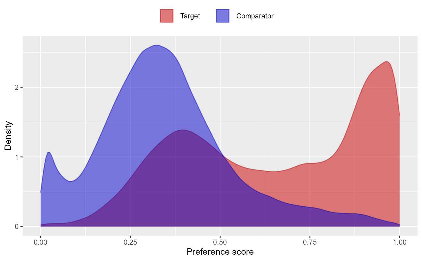
Note that some of the file names will appear several times in the table. For example, analysis 3 and 5 only differ in terms of the outcome model, and will share the same propensity score and stratification files.
We can always retrieve the file reference table again using the
getFileReference() function:
result <- getFileReference(folder)We can get a summary of the results using
getResultsSummary():
resultsSum <- getResultsSummary(folder)
resultsSum
## # A tibble: 216 × 27
## analysisId targetId comparatorId nestingCohortId outcomeId targetSubjects
## <int> <int> <int> <int> <int> <int>
## 1 1 1 2 3 77 86201
## 2 1 1 2 3 29735 88336
## 3 1 1 2 3 140673 83134
## 4 1 1 2 3 197494 89155
## 5 1 1 2 3 198185 89318
## 6 1 1 2 3 198199 88806
## 7 1 1 2 3 200528 88682
## 8 1 1 2 3 257315 88328
## 9 1 1 2 3 314658 79863
## 10 1 1 2 3 317376 89190
## # ℹ 206 more rows
## # ℹ 21 more variables: comparatorSubjects <int>, targetDays <dbl>,
## # comparatorDays <dbl>, targetOutcomes <dbl>, comparatorOutcomes <dbl>,
## # rr <dbl>, ci95Lb <dbl>, ci95Ub <dbl>, p <dbl>, oneSidedP <dbl>,
## # logRr <dbl>, seLogRr <dbl>, llr <dbl>, calibratedRr <dbl>,
## # calibratedCi95Lb <dbl>, calibratedCi95Ub <dbl>, calibratedP <dbl>,
## # calibratedOneSidedP <dbl>, calibratedLogRr <dbl>, …This tells us, per target-comparator-outcome-analysis combination, the estimated relative risk and 95% confidence interval, as well as the number of people in the treated and comparator group (after trimming and matching if applicable), and the number of outcomes observed for those groups within the specified risk windows.
Diagnostics
CohorMethod will have automatically executed a set of
diagnostics for each target-comparator-(nesting)-outcome:
- Equipoise: Pass if the equipoise is greater than 0.2, meaning the two cohorts are sufficiently comparable even before PS adjustment.
- Balance: Pass if the absolute standardized difference of means of all covariates is smaller than 0.1. We compute balance for both the shared balance (across all outcomes), and the per-outcome balance (which often only contains a small subset of covariates), and only pass if we pass for both.
- Generalizability: Pass if the standardized difference of means when comparing the analytic cohorts (e.g. after PS matching) to the original cohorts is smaller than some threshold for all covariates. We currently don’t set a threshold for this diagnostic, as we believe even less generalizable findings can still be meaningful.
- Systematic error: Pass is the expected absolute systematic error (EASE) is smaller than 0.25. EASE is computed by first fitting a normal distribution to the negative control estimates, and then integrating over the absolute value of this distribution. If EASE equals 0, all variation in negative control estimates can be explained by random error (as expressed in the confidence intervals) alone. Higher EASE scores indicate there is systematic error.
- Power: Pass if the minimum detectable relative risk is smaller than 10; We do not show estimates that have extremely low power because many people have trouble interpreting very wide confidence intervals. Underpowered estimates do still contribute to calibration, and when running across multiple databases, to the meta-analysis.
These diagnostics rely in threshold that can be specified using the
createCmDiagnosticThresholds(), which can be used in the
createCmAnalysesSpecifications() when invoking
runCmAnalyses().
Note that we are moving to balance diagnostic based on significance testing to avoid failing the balance diagnostics on smaller data sets. Currently the default is still to use the traditional balance approach.
We can retrieve the diagnostics:
diagnostics <- getDiagnosticsSummary(folder)
diagnostics
## # A tibble: 216 × 21
## analysisId targetId comparatorId nestingCohortId outcomeId maxSdm
## <int> <int> <int> <int> <int> <dbl>
## 1 1 1 2 3 77 NA
## 2 1 1 2 3 29735 NA
## 3 1 1 2 3 140673 NA
## 4 1 1 2 3 197494 NA
## 5 1 1 2 3 198185 NA
## 6 1 1 2 3 198199 NA
## 7 1 1 2 3 200528 NA
## 8 1 1 2 3 257315 NA
## 9 1 1 2 3 314658 NA
## 10 1 1 2 3 317376 NA
## # ℹ 206 more rows
## # ℹ 15 more variables: sdmFamilyWiseMinP <dbl>, balanceDiagnostic <chr>,
## # sharedMaxSdm <dbl>, sharedSdmFamilyWiseMinP <dbl>,
## # sharedBalanceDiagnostic <chr>, equipoise <dbl>, equipoiseDiagnostic <chr>,
## # generalizabilityMaxSdm <dbl>, generalizabilityDiagnostic <chr>, mdrr <dbl>,
## # mdrrDiagnostic <chr>, ease <dbl>, easeDiagnostic <chr>,
## # unblindForEvidenceSynthesis <lgl>, unblind <lgl>The ‘unblind’ column tells us whether we have passed all diagnostics. We can see for how many TCOs we pass diagnostics per analyses:
diagnostics |>
  group_by(analysisId) |>
  summarise(passing = sum(unblind))
## # A tibble: 6 × 2
## analysisId passing
## <int> <int>
## 1 1 0
## 2 2 27
## 3 3 0
## 4 4 0
## 5 5 27
## 6 6 0Here we see we pass diagnostics for many outcomes (including the negative controls) for both analyses using matching, but fail for all others. We can drill down into the diagnostics why this is (in this case we fail because we don’t achieve covariate balance).
Empirical calibration and negative control distribution
Because our study included negative control outcomes, our analysis summary also contains calibrated confidence intervals and p-values. We can also create the calibration effect plots for every analysis ID. In each plot, the blue dots represent our negative control outcomes, and the yellow diamond represents our health outcome of interest: GI bleed. An unbiased, well-calibrated analysis should have 95% of the negative controls between the dashed lines (ie. 95% should have p > .05).
install.packages("EmpiricalCalibration")
library(EmpiricalCalibration)

# Analysis 1: No matching, simple outcome model
ncs <- resultsSum |>
  filter(analysisId == 1,
         outcomeId != 77)
hoi <- resultsSum |>
  filter(analysisId == 1,
         outcomeId == 77)
null <- fitNull(ncs$logRr, ncs$seLogRr)
plotCalibrationEffect(logRrNegatives = ncs$logRr,
                      seLogRrNegatives = ncs$seLogRr,
                      logRrPositives = hoi$logRr,
                      seLogRrPositives = hoi$seLogRr, null)
# Analysis 2: Matching
ncs <- resultsSum |>
  filter(analysisId == 2,
         outcomeId != 77)
hoi <- resultsSum |>
  filter(analysisId == 2,
         outcomeId == 77)
null <- fitNull(ncs$logRr, ncs$seLogRr)
plotCalibrationEffect(logRrNegatives = ncs$logRr,
                      seLogRrNegatives = ncs$seLogRr,
                      logRrPositives = hoi$logRr,
                      seLogRrPositives = hoi$seLogRr, null)
# Analysis 3: Stratification
ncs <- resultsSum |>
  filter(analysisId == 3,
         outcomeId != 77)
hoi <- resultsSum |>
  filter(analysisId == 3,
         outcomeId == 77)
null <- fitNull(ncs$logRr, ncs$seLogRr)
plotCalibrationEffect(logRrNegatives = ncs$logRr,
                      seLogRrNegatives = ncs$seLogRr,
                      logRrPositives = hoi$logRr,
                      seLogRrPositives = hoi$seLogRr, null)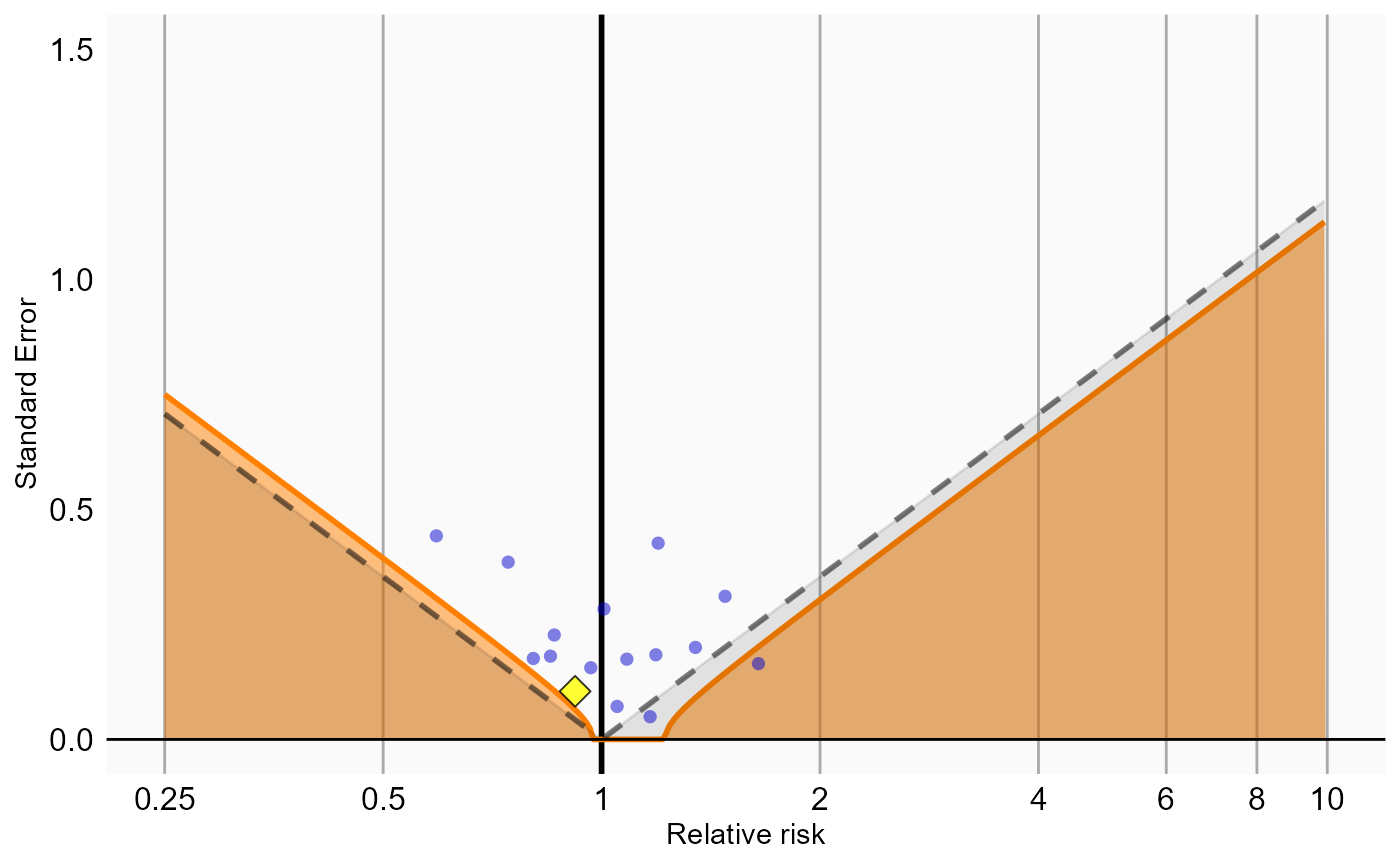
# Analysis 4: Inverse probability of treatment weighting
ncs <- resultsSum |>
  filter(analysisId == 4,
         outcomeId != 77)
hoi <- resultsSum |>
  filter(analysisId == 4,
         outcomeId == 77)
null <- fitNull(ncs$logRr, ncs$seLogRr)
plotCalibrationEffect(logRrNegatives = ncs$logRr,
                      seLogRrNegatives = ncs$seLogRr,
                      logRrPositives = hoi$logRr,
                      seLogRrPositives = hoi$seLogRr, null)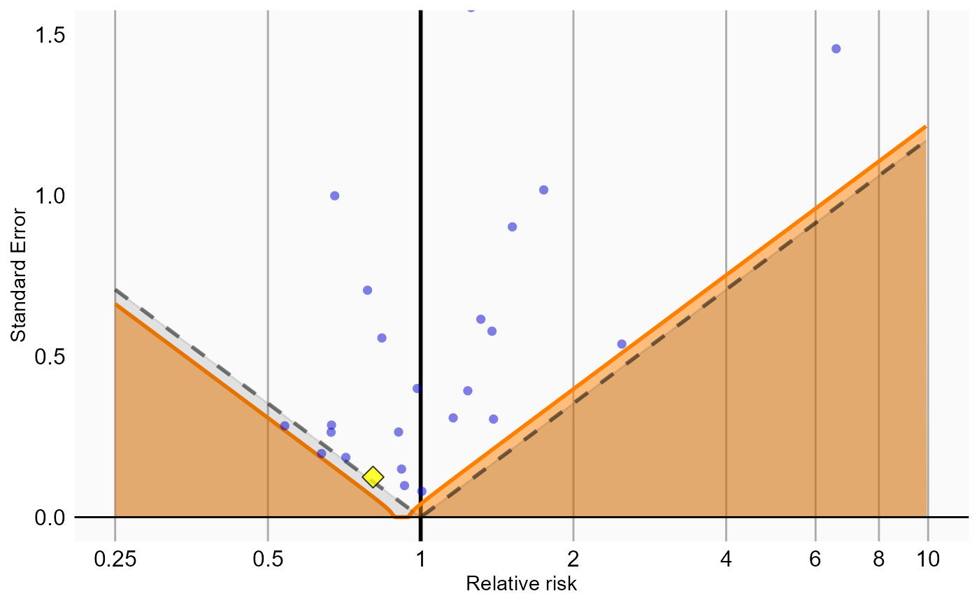
# Analysis 5: Stratification plus full outcome model
ncs <- resultsSum |>
  filter(analysisId == 5,
         outcomeId != 77)
hoi <- resultsSum |>
  filter(analysisId == 5,
         outcomeId == 77)
null <- fitNull(ncs$logRr, ncs$seLogRr)
plotCalibrationEffect(logRrNegatives = ncs$logRr,
                      seLogRrNegatives = ncs$seLogRr,
                      logRrPositives = hoi$logRr,
                      seLogRrPositives = hoi$seLogRr, null)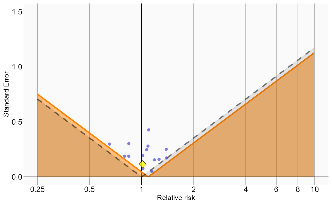
Analysis 6 explored interactions with certain variables. The estimates for these interaction terms are stored in a separate results summary. We can examine whether these estimates are also consistent with the null. In this example we consider the interaction with ‘concurrent use of antithrombotic agents’ (covariate ID 21600960413):
interactionResultsSum <- getInteractionResultsSummary(folder)

# Analysis 6: Stratification plus interaction terms
ncs <- interactionResultsSum |>
  filter(analysisId == 6,
         interactionCovariateId == 21600960413,
         outcomeId != 77)
hoi <- interactionResultsSum |>
  filter(analysisId == 6,
         interactionCovariateId == 21600960413,
         outcomeId == 77)
null <- fitNull(ncs$logRr, ncs$seLogRr)
plotCalibrationEffect(logRrNegatives = ncs$logRr,
                      seLogRrNegatives = ncs$seLogRr,
                      logRrPositives = hoi$logRr,
                      seLogRrPositives = hoi$seLogRr, null)
## Warning in fitNull(ncs$logRr, ncs$seLogRr): Estimate(s) with extreme logRr
## detected: abs(logRr) > log(100). Removing before fitting null distribution## Warning in checkWithinLimits(yLimits, c(seLogRrNegatives, seLogRrPositives), :
## Values are outside plotted range. Consider adjusting yLimits parameter## Warning in checkWithinLimits(log(xLimits), c(logRrNegatives, logRrPositives), :
## Values are outside plotted range. Consider adjusting xLimits parameter## Warning: Removed 1 row containing missing values or values outside the scale range
## (`geom_vline()`).## Warning: Removed 1 row containing missing values or values outside the scale range
## (`geom_point()`).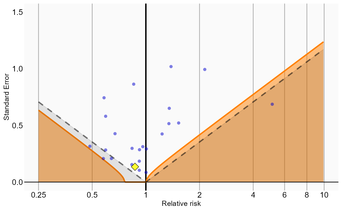
Exporting to CSV
The results generated so far all reside in binary object on your
local file system, mixing aggregate statistics such as hazard ratios
with patient-level data including propensity scores per person. How
could we share our results with others, possibly outside our
organization? This is where the exportToCsv() function
comes in. This function exports all results, including diagnostics to
CSV (comma-separated values) files. These files only contain aggregate
statistics, not patient-level data. The format is CSV files to enable
human review.
exportToCsv(
  folder,
  exportFolder = file.path(folder, "export"),
  databaseId = "My CDM",
  minCellCount = 5,
  maxCores = parallel::detectCores()
)
Any person counts in the results that are smaller than the
minCellCount argument will be blinded, by replacing the
count with the negative minCellCount. For example, if the
number of people with the outcome is 3, and
minCellCount = 5, the count will be reported to be -5,
which in the Shiny app will be displayed as ‘<5’.
Information on the data model used to generate the CSV files can be
retrieved using getResultsDataModelSpecifications():
## # A tibble: 191 × 8
##    tableName   columnName dataType isRequired primaryKey minCellCount deprecated
##    <chr>       <chr>      <chr>    <chr>      <chr>      <chr>        <chr>
##  1 cm_attriti… sequence_… int      Yes        Yes        No           No
##  2 cm_attriti… descripti… varchar  Yes        No         No           No
##  3 cm_attriti… subjects   int      Yes        No         Yes          No
##  4 cm_attriti… exposure_… bigint   Yes        Yes        No           No
##  5 cm_attriti… target_co… bigint   Yes        Yes        No           No
##  6 cm_attriti… analysis_… int      Yes        Yes        No           No
##  7 cm_attriti… outcome_id bigint   Yes        Yes        No           No
##  8 cm_attriti… database_… varchar  Yes        Yes        No           No
##  9 cm_follow_… target_co… bigint   Yes        Yes        No           No
## 10 cm_follow_… outcome_id bigint   Yes        Yes        No           No
## # ℹ 181 more rows
## # ℹ 1 more variable: description <chr>
Acknowledgments
Considerable work has been dedicated to provide the
CohortMethod package.
citation("CohortMethod")## To cite CohortMethod in publications use:
##
## Schuemie MJ, Reps JM, Black A, DeFalco F, Evans L, Fridgeirsson E,
## Gilbert JP, Knoll C, Lavallee M, Rao G, Rijnbeek P, Sadowski K, Sena
## A, Swerdel J, Williams RD, Suchard MA (2024). "Health-analytics data
## to evidence suite (HADES): open-source software for observational
## research." _Studies in Health Technology and Informatics_, *310*,
## 966-970. doi:10.3233/SHTI231108 <https://doi.org/10.3233/SHTI231108>,
## <https://doi.org/10.3233/shti231108>.
##
## A BibTeX entry for LaTeX users is
##
## @Article{,
## title = {Health-analytics data to evidence suite (HADES): open-source software for observational research},
## author = {M. J. Schuemie and J. M. Reps and A. Black and F. DeFalco and L. Evans and E. Fridgeirsson and J. P. Gilbert and C. Knoll and M. Lavallee and G. Rao and P. Rijnbeek and K. Sadowski and A. Sena and J. Swerdel and R. D. Williams and M. A. Suchard},
## journal = {Studies in Health Technology and Informatics},
## year = {2024},
## volume = {310},
## pages = {966-970},
## doi = {10.3233/SHTI231108},
## url = {https://doi.org/10.3233/shti231108},
## }Further, CohortMethod makes extensive use of the
Cyclops package.
citation("Cyclops")## To cite Cyclops in publications use:
##
## Suchard MA, Simpson SE, Zorych I, Ryan P, Madigan D (2013). "Massive
## parallelization of serial inference algorithms for complex
## generalized linear models." _ACM Transactions on Modeling and
## Computer Simulation_, *23*, 10. doi:10.1145/2414416.2414791
## <https://doi.org/10.1145/2414416.2414791>.
##
## A BibTeX entry for LaTeX users is
##
## @Article{,
## author = {M. A. Suchard and S. E. Simpson and I. Zorych and P. Ryan and D. Madigan},
## title = {Massive parallelization of serial inference algorithms for complex generalized linear models},
## journal = {ACM Transactions on Modeling and Computer Simulation},
## volume = {23},
## pages = {10},
## year = {2013},
## doi = {10.1145/2414416.2414791},
## }This work is supported in part through the National Science Foundation grant IIS 1251151.