Running the OHDSI Methods Benchmark

Introduction

When designing an observational study, there are many study designs to choose from, and many additional choices to make, and it is often unclear how these choices will affect the accuracy of the results. (e.g. If I match on propensity scores, will that lead to more or less bias than when I stratify? What about power?) The literature contains many papers evaluating one design choice at a time, but often with unsatisfactory scientific rigor; typically, a method is evaluated on one or two exemplar study from which we cannot generalize, or by using simulations which have an unclear relationship with the real world.

This vignette describes the OHDSI Methods Benchmark for evaluating population-level estimation methods, a benchmark that can inform on how a particular study design and set of analysis choices perform in general. The benchmark consists of a gold standard of research hypothesis where the truth is known, and a set of metrics for characterizing a methods performance when applied to the gold standard. We distinguish between two types of tasks: (1) estimation of the average effect of an exposure on an outcome relative to no exposure (effect estimation), and (2) estimation of the average effect of an exposure on an outcome relative to another exposure (comparative effect estimation). The benchmark allows evaluation of a method on either or both tasks.

This benchmark builds on previous efforts in EU-ADR, OMOP, and the WHO, adding the ability to evaluate methods on both tasks, and using synthetic positive controls as real positive controls have been observed to be problematic in the past.

Gold standard

The gold standard comprises 800 entries, with each item specifying a target exposure, comparator exposure, outcome, nesting cohort, and true effect size. The true effect size refers to the absolute effect of the target on the outcome. Because the comparator is always believed to have no effect on the outcome, the true effect size also holds for the relative effect of the target compared to the comparator. Thus, each entry can be used for evaluating both effect estimation and comparative effect estimation. The nesting cohort identifies a more homogeneous subgroup of the population and can be used to evaluate methods such as the nested case-control design.

Of the total set, 200 entries are real negative controls with a presumed true relative risk of 1. We select these negative controls by first picking four diverse outcomes (acute pancreatitis, gastrointestinal bleeding, inflammatory bowel disease, and stroke) and four diverse exposures (ciprofloxacin, diclofenac, metformin, and sertraline). For each of the four outcomes, we create 25 entries with target and comparator exposures that are not believed to cause the outcome. To aid the creation of these entries, we generate candidate lists of negative controls for each of the four main outcomes and four main exposures using an automated procedure, drawing on literature, product labels, and spontaneous reports. These candidates are used to construct target-comparator-outcome triplets where neither the target nor the exposure causes the outcome, and the target and comparator were either previously compared in a randomized trial per ClinicalTrials.gov, or both had the same four-digit ATC code (same indication) but not the same five-digit ATC code (different class). These candidates are ranked on prevalence of the exposures and outcome and manually reviewed until 25 were approved per initial outcome or exposure. Nesting cohorts were selected by manually reviewing the most prevalent conditions and procedures on the first day of the target or comparator treatment.

The remaining 600 entries are positive controls, which were automatically derived from the 200 negative controls by adding synthetic additional outcomes during the target exposure until a desired incidence rate ratio was achieved between before and after injection of the synthetic outcomes. The target incidence rate ratios were 1.25, 2, and 4. To preserve (measured) confounding, predictive models were fitted for each outcome during target exposure and used to generate probabilities from which the synthetic outcomes were sampled.

Metrics

Once a method has been used to produce estimates for the gold standard the following metrics are computed:

AUC: the ability to discriminate between positive controls and negative controls.
Coverage: how often the true effect size is within the 95% confidence interval.
Mean precision: Precision is computed as 1 / (standard error)2, higher precision means narrower confidence intervals. We use the geometric mean to account for the skewed distribution of the precision.
Mean squared error (MSE): Mean squared error between the log of the effect size point-estimate and the log of the true effect size.
Type 1 error: For negative controls, how often was the null rejected (at alpha = 0.05). This is equivalent to the false positive rate and 1 - specificity.
Type 2 error: For positive controls, how often was the null not rejected (at alpha = 0.05). This is equivalent to the false negative rate and 1 - sensitivity.
Non-estimable: For how many of the controls was the method unable to produce an estimate? There can be various reasons why an estimate cannot be produced, for example because there were no subjects left after propensity score matching, or because no subjects remained having the outcome.

The Benchmark computes these metrics both overall, as well as stratified by true effect size, by each of the four initial outcomes and four initial exposures, and by amount of data as reflected by the minimum detectable relative risk (MDRR). When a method cannot estimate an effect, it returns an estimate of 1 with an infinite confidence interval.

In prior work we described a method for empirically calibrating p-values and confidence intervals. Briefly, empirical calibration estimates a systematic error distribution based on the estimates produced for the negative and positive controls. This systematic error is then taken into consideration, in addition to the random error, when computing the confidence interval and p-value. We therefore also report the performance metrics listed above after calibration, using a leave-one-out approach: for each control the error distributions are fitted on all controls except the control being calibrated and its siblings. By siblings we mean the set of a negative control and the positive controls derived from that negative control.

Running the benchmark

This section will describe how to run methods against the benchmark on a particular observational healthcare database. The database needs to conform to the OMOP Common Data Model (CDM).

Specifying locations on the server and local file system

We need to specify the following locations on the database server:

The database schema containing the observational healthcare data in CDM format. Only read access is required to this schema.
A database schema and table name where outcome cohorts can be instantiated. Write access is required to this schema.
A database schema and table name where nesting cohorts can be instantiated. Write access is required to this schema.
On Oracle only: a schema where temporary tables can be created. Write access is required to this schema. This is required since Oracle doesn’t fully support temp tables like other database platforms.

We also need to specify on the local file system:

An output folder where all intermediary and final results can be written. This should not be a network drive, since that would severely slow down the analyses.

Below is example code showing we specify how to connect to the database server, and the various required locations. MethodEvaluation uses the DatabaseConnector package, which provides the createConnectionDetails function. Type ?createConnectionDetails for the specific settings required for the various database management systems (DBMS).

library(MethodEvaluation)
connectionDetails <- createConnectionDetails(
  dbms = "postgresql",
  server = "localhost/ohdsi",
  user = "joe",
  password = "supersecret"
)

cdmDatabaseSchema <- "my_cdm_data"
oracleTempSchema <- NULL
outcomeDatabaseSchema <- "scratch"
outcomeTable <- "ohdsi_outcomes"
nestingCohortDatabaseSchema <- "scratch"
nestingCohortTable <- "ohdsi_nesting_cohorts"
outputFolder <- "/home/benchmarkOutput"
cdmVersion <- "5"

Note that for Microsoft SQL Server, database schemas need to specify both the database and the schema, so for example cdmDatabaseSchema <- "my_cdm_data.dbo".

Creating all necessary cohorts

In order to run our population-level effect estimation method, we will need to identify the exposures and outcomes of interest. To identify exposures we will simlpy use the predefined exposure eras in the drug_era table in the CDM. However, for the outcomes custom cohorts need to be generated. In addition, some methods such as the nested case-control design require nesting cohorts to be defined. The negative control outcome and nesting cohorts can be generated using the following command:

createReferenceSetCohorts(
  connectionDetails = connectionDetails,
  oracleTempSchema = oracleTempSchema,
  cdmDatabaseSchema = cdmDatabaseSchema,
  outcomeDatabaseSchema = outcomeDatabaseSchema,
  outcomeTable = outcomeTable,
  nestingDatabaseSchema = nestingCohortDatabaseSchema,
  nestingTable = nestingCohortTable,
  referenceSet = "ohdsiMethodsBenchmark"
)

This will automatically create the outcome and nesting cohort tables, and populate them.

The nest step is to create the positive controls. These are generated by taking the negative controls, and adding synthetic outcomes during exposed time to achieve predefined relative risks greater than one. The synthetic outcomes are sampled based on models that are fitted for each negative control outcome, using predictors extracted from the data. These positive control outcomes are added to the outcome table.

synthesizeReferenceSetPositiveControls(
  connectionDetails = connectionDetails,
  oracleTempSchema = oracleTempSchema,
  cdmDatabaseSchema = cdmDatabaseSchema,
  outcomeDatabaseSchema = outcomeDatabaseSchema,
  outcomeTable = outcomeTable,
  maxCores = 10,
  workFolder = outputFolder,
  summaryFileName = file.path(
    outputFolder,
    "allControls.csv"
  ),
  referenceSet = "ohdsiMethodsBenchmark"
)

Fitting the outcome models can take a while. It is recommend to set the maxCores argument to the number of CPU cores available in the machine to speed up the process. Note that at the end, a file will be created called allControls.csv in the output folder containing the information on the controls:

allControls <- read.csv(file.path(outputFolder, "allControls.csv"))
head(allControls)

#>  outcomeId comparatorId targetId targetName comparatorName nestingId                  nestingName        outcomeName             type targetEffectSize trueEffectSize trueEffectSizeFirstExposure oldOutcomeId mdrrTarget
#> 1         1      1105775  1110942 omalizumab  Aminophylline  37203741 Bronchospasm and obstruction Acute pancreatitis Exposure control                1              1                           1            1   1.421960
#> 2         1      1110942  1140088 Dyphylline     omalizumab  37203741 Bronchospasm and obstruction Acute pancreatitis Exposure control                1              1                           1            1   1.420173
#> 3         1      1136422   943634 epinastine levocetirizine  36009773            Rhinitis allergic Acute pancreatitis Exposure control                1              1                           1            1   1.217681
#> 4         1      1315865 40163718  prasugrel   fondaparinux  37622411              Phlebosclerosis Acute pancreatitis Exposure control                1              1                           1            1   1.196514
#> 5         1      1315865  1350310 cilostazol   fondaparinux  37622411              Phlebosclerosis Acute pancreatitis Exposure control                1              1                           1            1   1.233415
#> 6         1      1336926  1311276 vardenafil      tadalafil  36919202           Sexual dysfunction Acute pancreatitis Exposure control                1              1                           1            1   1.097112
#>   mdrrComparator
#> 1       1.177202
#> 2       1.421960
#> 3       1.085877
#> 4       1.278911
#> 5       1.278911
#> 6       1.060737

Running the method to evaluate

Now that we have the controls in place, we can run the method we would like to evaluate. Here we will run the SelfControlledCohort package which implements the Self-Controlled Cohort (SCC) design. We first will first define some SCC analysis settings to evaluate. Here we define two analysis settings, one using the length of exposure as the time-at-risk, and one using the first 30 days after exposure start as the time-at-risk:

library(SelfControlledCohort)
runSccArgs1 <- createRunSelfControlledCohortArgs(
  addLengthOfExposureExposed = TRUE,
  riskWindowStartExposed = 0,
  riskWindowEndExposed = 0,
  riskWindowEndUnexposed = -1,
  addLengthOfExposureUnexposed = TRUE,
  riskWindowStartUnexposed = -1,
  washoutPeriod = 365
)

sccAnalysis1 <- createSccAnalysis(
  analysisId = 1,
  description = "Length of exposure",
  runSelfControlledCohortArgs = runSccArgs1
)

runSccArgs2 <- createRunSelfControlledCohortArgs(
  addLengthOfExposureExposed = FALSE,
  riskWindowStartExposed = 0,
  riskWindowEndExposed = 30,
  riskWindowEndUnexposed = -1,
  addLengthOfExposureUnexposed = FALSE,
  riskWindowStartUnexposed = -30,
  washoutPeriod = 365
)

sccAnalysis2 <- createSccAnalysis(
  analysisId = 2,
  description = "30 days of each exposure",
  runSelfControlledCohortArgs = runSccArgs2
)
sccAnalysisList <- list(sccAnalysis1, sccAnalysis2)

Next, we specify all exposure-outcome pairs we want to apply the SCC design to. Note that we only use the targetId and outcomeId fields of the controls, because the SCC design can only be used for effect estimation, and does not support nesting:

allControls <- read.csv(file.path(outputFolder, "allControls.csv"))
eos <- list()
for (i in 1:nrow(allControls)) {
  eos[[length(eos) + 1]] <- createExposureOutcome(
    exposureId = allControls$targetId[i],
    outcomeId = allControls$outcomeId[i]
  )
}

Then, we run the SCC method. The following command will execute the SCC with the specified analysis settings against the exposure-outcome pairs:

sccResult <- runSccAnalyses(
  connectionDetails = connectionDetails,
  cdmDatabaseSchema = cdmDatabaseSchema,
  oracleTempSchema = oracleTempSchema,
  exposureTable = "drug_era",
  outcomeDatabaseSchema = outcomeDatabaseSchema,
  outcomeTable = outcomeTable,
  sccAnalysisList = sccAnalysisList,
  exposureOutcomeList = eos,
  outputFolder = outputFolder
)
sccSummary <- summarizeAnalyses(sccResult, outputFolder)
write.csv(sccSummary, file.path(outputFolder, "sccSummary.csv"), row.names = FALSE)

This produces a file called sccSummary.csv which contains the effect size estimates for each analysisId-exposureId-outcomeId combination.

Packaging the evaluation results

Now that we have the estimates, we need to feed them back into the MethodEvaluation package. To do that we need to create two data frames, one specifying the effect size estimates, the other providing details on the various analyses.

First, we specify the estimates:

estimates <- readRDS(file.path(outputFolder, "sccSummary.csv"))
estimates <- data.frame(
  analysisId = estimates$analysisId,
  targetId = estimates$exposureId,
  outcomeId = estimates$outcomeId,
  logRr = estimates$logRr,
  seLogRr = estimates$seLogRr,
  ci95Lb = estimates$irrLb95,
  ci95Ub = estimates$irrUb95
)
head(estimates)

#>   analysisId targetId outcomeId      logRr   seLogRr    ci95Lb    ci95Ub
#> 1          1  1110942         1 -1.5000000        NA        NA 13.177433
#> 2          1  1140088         1         NA        NA        NA        NA
#> 3          1   943634         1         NA        NA        NA        NA
#> 4          1 40163718         1 -0.4054651 0.6926191 0.1479317  2.234489
#> 5          1  1350310         1 -0.2876821 0.7038381 0.1642789  2.592973
#> 6          1  1311276         1 -0.1823216 0.5451585 0.2651910  2.247182

Next, we create the analysis reference:

# Create a reference of the analysis settings:
analysisRef <- data.frame(
  method = "SelfControlledCohort",
  analysisId = c(1, 2),
  description = c(
    "Length of exposure",
    "30 days of each exposure"
  ),
  details = "",
  comparative = FALSE,
  nesting = FALSE,
  firstExposureOnly = FALSE
)
head(analysisRef)

#>                 method analysisId              description details comparative
#> 1 SelfControlledCohort          1       Length of exposure               FALSE
#> 2 SelfControlledCohort          2 30 days of each exposure               FALSE
#>   nesting firstExposureOnly
#> 1   FALSE             FALSE
#> 2   FALSE             FALSE

Finally, we supply these two data frames, together with the data frame with controls to the packageOhdsiBenchmarkResults function:

allControls <- read.csv(file.path(outputFolder, "allControls.csv"))
packageOhdsiBenchmarkResults(
  estimates = estimates,
  controlSummary = allControls,
  analysisRef = analysisRef,
  databaseName = databaseName,
  exportFolder = file.path(outputFolder, "export")
)

This will generate two CSV files in the export folder. Results from different methods and databases can all be written to the same export folder.

Computing metrics

There are two ways to view the method’s performance metrics: using a Shiny app, and by generating a data frame.

Using the Shiny app

Run the follow command to launch the Shiny app and view the metrics:

exportFolder <- file.path(outputFolder, "export")
launchMethodEvaluationApp(exportFolder)

This will launch a Shiny app as shown in Figure 1.

Method Benchmark Shiny app

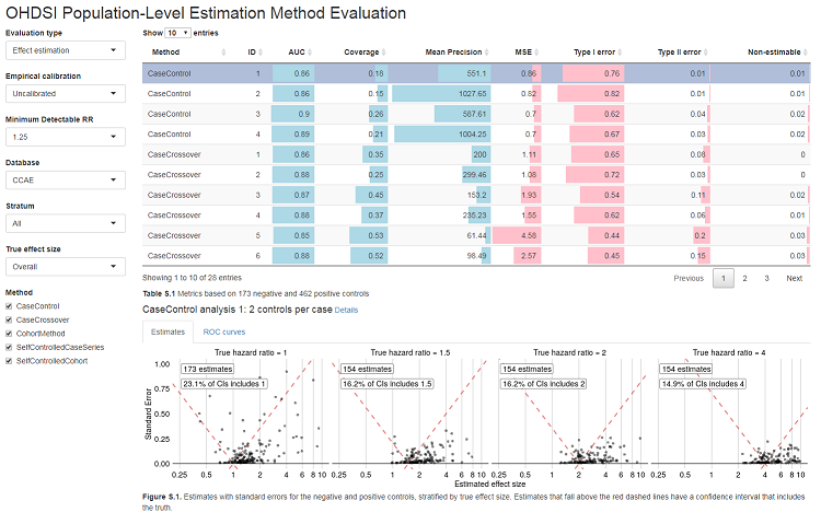
Note that the export folder can hold results from multiple methods and multiple databases.

Generating a data frame

Alternatively, we can output the metrics to a data frame:

exportFolder <- file.path(outputFolder, "export")
metrics <- computeOhdsiBenchmarkMetrics(exportFolder,
  mdrr = 1.25,
  stratum = "All",
  trueEffectSize = "Overall",
  calibrated = FALSE,
  comparative = FALSE
)
head(metrics)

#>    database               method analysisId                                           description  auc coverage   meanP  mse type1 type2 nonEstimable
#> 1     CCAE SelfControlledCohort          1                    Length of exposure 0.89     0.21 1048.97 0.30  0.66  0.08         0.01
#> 2     CCAE SelfControlledCohort          2                        30 days of each exposure 0.87     0.41  422.25 0.14  0.55  0.11         0.00

See ?computeOhdsiBenchmarkMetrics for information on the various arguments.

Martijn J. Schuemie

2023-06-30