Summarise concept counts
Source:vignettes/B-summarise_concept_set_counts.Rmd
B-summarise_concept_set_counts.RmdIntroduction
In this vignette, we will explore the OmopSketch functions
designed to provide information about the number of counts of specific
concepts. Specifically, there are two key functions that facilitate
this, summariseConceptSetCounts() and
plotConceptCounts(). The former one creates a summary
statistics results with the number of counts per each concept, and the
latter one creates a histogram plot.
Create a mock cdm
Let’s see an example of the previous functions. To start with, we will load essential packages and create a mock cdm using Eunomia database.
library(dplyr)
#>
#> Attaching package: 'dplyr'
#> The following objects are masked from 'package:stats':
#>
#>     filter, lag
#> The following objects are masked from 'package:base':
#>
#>     intersect, setdiff, setequal, union
library(CDMConnector)
library(DBI)
library(duckdb)
library(OmopSketch)
library(CodelistGenerator)

# Connect to Eunomia database
con <- DBI::dbConnect(duckdb::duckdb(), CDMConnector::eunomiaDir())
cdm <- CDMConnector::cdmFromCon(
  con = con, cdmSchema = "main", writeSchema = "main"
)
#> Note: method with signature 'DBIConnection#Id' chosen for function 'dbExistsTable',
#>  target signature 'duckdb_connection#Id'.
#>  "duckdb_connection#ANY" would also be valid
#> ! cdm name not specified and could not be inferred from the cdm source table

cdm
#>
#> ── # OMOP CDM reference (duckdb) of An OMOP CDM database ───────────────────────
#> • omop tables: person, observation_period, visit_occurrence, visit_detail,
#> condition_occurrence, drug_exposure, procedure_occurrence, device_exposure,
#> measurement, observation, death, note, note_nlp, specimen, fact_relationship,
#> location, care_site, provider, payer_plan_period, cost, drug_era, dose_era,
#> condition_era, metadata, cdm_source, concept, vocabulary, domain,
#> concept_class, concept_relationship, relationship, concept_synonym,
#> concept_ancestor, source_to_concept_map, drug_strength
#> • cohort tables: -
#> • achilles tables: -
#> • other tables: -
Summarise concept counts
First, let’s generate a list of codes for the concept
dementia using CodelistGenerator
package.
acetaminophen <- getCandidateCodes(
  cdm = cdm,
  keywords = "acetaminophen",
  domains = "Drug",
  includeDescendants = TRUE
) |>
  dplyr::pull("concept_id")
#> Limiting to domains of interest
#> Getting concepts to include
#> Adding descendants
#> Search completed. Finishing up.
#> ✔ 7 candidate concepts identified
#>
#> Time taken: 0 minutes and 0 seconds

sinusitis <- getCandidateCodes(
  cdm = cdm,
  keywords = "sinusitis",
  domains = "Condition",
  includeDescendants = TRUE
) |>
  dplyr::pull("concept_id")
#> Limiting to domains of interest
#> Getting concepts to include
#> Adding descendants
#> Search completed. Finishing up.
#> ✔ 4 candidate concepts identified
#>
#> Time taken: 0 minutes and 0 seconds
Now we want to explore the occurrence of these concepts within the
database. For that, we can use summariseConceptSetCounts()
from OmopSketch:
summariseConceptSetCounts(cdm,
                       conceptSet = list("acetaminophen" = acetaminophen,
                                        "sinusitis" = sinusitis)) |>
  select(group_level, variable_name, variable_level, estimate_name, estimate_value) |>
  glimpse()
#> ℹ Searching concepts from domain drug in drug_exposure.
#> ℹ Searching concepts from domain condition in condition_occurrence.
#> ℹ Counting concepts
#> Rows: 24
#> Columns: 5
#> $ group_level    <chr> "acetaminophen", "acetaminophen", "sinusitis", "sinusit…
#> $ variable_name  <chr> "Number records", "Number subjects", "Number records", …
#> $ variable_level <chr> NA, NA, NA, NA, NA, NA, NA, NA, NA, NA, NA, NA, NA, NA,…
#> $ estimate_name  <chr> "count", "count", "count", "count", "count", "count", "…
#> $ estimate_value <chr> "14205", "2679", "20033", "2689", "2158", "1428", "306"…
By default, the function will provide information about either the
number of records (estimate_name == "record_count") for
each concept_id or the number of people
(estimate_name == "person_count"):
summariseConceptSetCounts(cdm,
                       conceptSet = list("acetaminophen" = acetaminophen,
                                        "sinusitis" = sinusitis),
                       countBy = c("record","person")) |>
  select(group_level, variable_name, estimate_name) |>
  distinct() |>
  arrange(group_level, variable_name)
#> ℹ Searching concepts from domain drug in drug_exposure.
#> ℹ Searching concepts from domain condition in condition_occurrence.
#> ℹ Counting concepts
#> # A tibble: 4 × 3
#>   group_level   variable_name   estimate_name
#>   <chr>         <chr>           <chr>
#> 1 acetaminophen Number records  count
#> 2 acetaminophen Number subjects count
#> 3 sinusitis     Number records  count
#> 4 sinusitis     Number subjects count
However, we can specify which one is of interest using
countBy argument:
summariseConceptSetCounts(cdm,
                       conceptSet = list("acetaminophen" = acetaminophen,
                                        "sinusitis" = sinusitis),
                       countBy = "record") |>
  select(group_level, variable_name, estimate_name) |>
  distinct() |>
  arrange(group_level, variable_name)
#> ℹ Searching concepts from domain drug in drug_exposure.
#> ℹ Searching concepts from domain condition in condition_occurrence.
#> ℹ Counting concepts
#> # A tibble: 2 × 3
#>   group_level   variable_name  estimate_name
#>   <chr>         <chr>          <chr>
#> 1 acetaminophen Number records count
#> 2 sinusitis     Number records count
One can further stratify by year, sex or age group using the
year, sex, and ageGroup
arguments.
summariseConceptSetCounts(cdm,
                       conceptSet = list("acetaminophen" = acetaminophen,
                                        "sinusitis" = sinusitis),
                       countBy = "person",
                       interval = "years",
                       sex  = TRUE,
                       ageGroup = list("<=50" = c(0,50), ">50" = c(51,Inf))) |>
  select(group_level, strata_level, variable_name, estimate_name) |>   glimpse()
#> ℹ Searching concepts from domain drug in drug_exposure.
#> ℹ Searching concepts from domain condition in condition_occurrence.
#> ℹ Counting concepts
#> Rows: 7,545
#> Columns: 4
#> $ group_level   <chr> "sinusitis", "acetaminophen", "acetaminophen", "sinusiti…
#> $ strata_level  <chr> "overall", "overall", "<=50", "<=50", ">50", ">50", "Fem…
#> $ variable_name <chr> "Number subjects", "Number subjects", "Number subjects",…
#> $ estimate_name <chr> "count", "count", "count", "count", "count", "count", "c…
Visualise the results
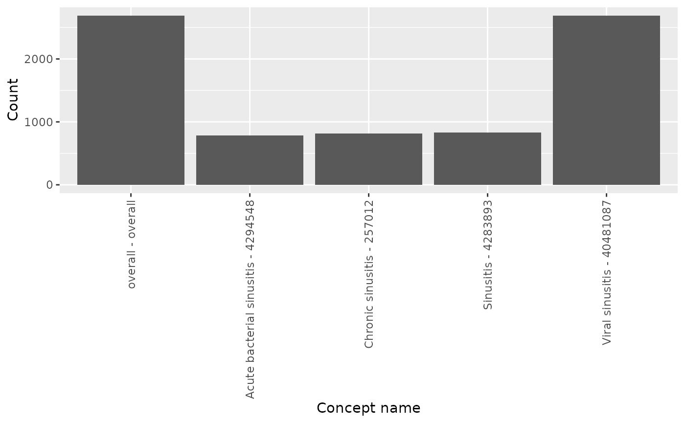
Finally, we can visualise the concept counts using
plotRecordCounts().
summariseConceptSetCounts(cdm,
                       conceptSet = list("sinusitis" = sinusitis),
                       countBy = "person") |>
  plotConceptSetCounts()
#> ℹ Searching concepts from domain condition in condition_occurrence.
#> ℹ Counting concepts
Notice that either person counts or record counts can be plotted. If
both have been included in the summarised result, you will have to
filter to only include one variable at time:
summariseConceptSetCounts(cdm,
                       conceptSet = list("sinusitis" = sinusitis),
                       countBy = c("person","record")) |>
  filter(variable_name == "Number subjects") |>
  plotConceptSetCounts()
#> ℹ Searching concepts from domain condition in condition_occurrence.
#> ℹ Counting concepts
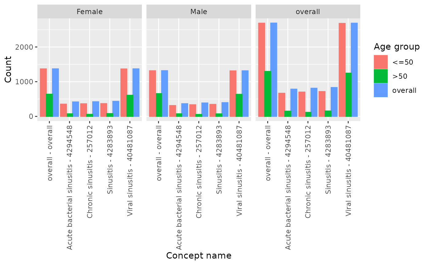
Additionally, if results were stratified by year, sex or age group,
we can further use facet or colour arguments
to highlight the different results in the plot. To help us identify by
which variables we can colour or facet by, we can use visOmopResult
package.
summariseConceptSetCounts(cdm,
                       conceptSet = list("sinusitis" = sinusitis),
                       countBy = c("person"),
                       sex = TRUE,
                       ageGroup = list("<=50" = c(0,50), ">50" = c(51, Inf))) |>
  visOmopResults::tidyColumns()
#> ℹ Searching concepts from domain condition in condition_occurrence.
#> ℹ Counting concepts
#>  [1] "cdm_name"              "codelist_name"         "age_group"
#>  [4] "sex"                   "variable_name"         "variable_level"
#>  [7] "count"                 "standard_concept_name" "standard_concept_id"
#> [10] "source_concept_name"   "source_concept_id"     "domain_id"

summariseConceptSetCounts(cdm,
                       conceptSet = list("sinusitis" = sinusitis),
                       countBy = c("person"),
                       sex = TRUE,
                       ageGroup = list("<=50" = c(0,50), ">50" = c(51, Inf))) |>
  plotConceptSetCounts(facet = "sex", colour = "age_group")
#> ℹ Searching concepts from domain condition in condition_occurrence.
#> ℹ Counting concepts