Plotting learning curves

Peter R. Rijnbeek, Xiaoyong Pan, Luis H. John, Jenna Reps

May 22, 2018

Introduction

Prediction models will show overly-optimistic performance when predicting on the same data as used for training. Therefore, we generally partition our data into a training set and testing set. We then train our prediction model on the training set portion and asses its ability to generalize to unseen data by measuring its performance on the testing set.

Learning curves inform about the effect of training set size on model performance by training a sequence of prediction models on successively larger subsets of the training set. A learning curve plot can also help in diagnosing a bias or variance problem. Learning curves objects can be created and plotted with the PatientLevelPrediction package.

Background

Figure 1 shows a commonly observed learning curve plot, where model performance is mapped to the vertical axis and training set size is mapped to the horizontal axis. If training set size is small, the performance on the training set is high, because a model can generally be fitted well to a limited number of training examples. At the same time, the performance on the testing set will be poor, because the model trained on such a limited number of training examples will not generalize well to unseen data in the testing set. As the training set size increases, the performance of the model on the training set will decrease. It becomes more difficult for the model to find a good fit through all the training examples. Also, the model will be trained on a more representative portion of training examples, making it generalize better to unseen data. This can be observed by the testing set performance increasing.

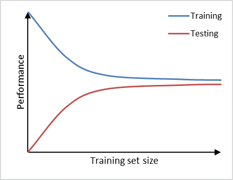
Figure 1. Learning curve plot with model performance mapped to the vertical axis and training set size mapped to the horizontal axis.

Bias and variance

We can observe high variance (overfitting) in a prediction model if it performs well on the training set, but poorly on the testing set (Figure 2). Adding additional data is a common approach to counteract high variance. From the learning curve it becomes apparent, that adding additional data may improve performance on the testing set a little further, as the learning curve has not yet plateaued and, thus, the model is not saturated yet. Therefore, adding more data will decrease the gap between training set and testing set, which is the main indicator for a high variance problem.

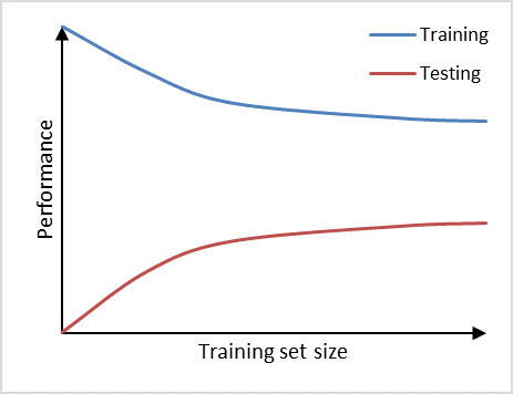
Figure 2. Prediction model suffering from high variance.

Furthermore, we can observe high bias (underfitting) if a prediction model performs poorly on the training set as well as on the testing set (Figure 3). The learning curves of training set and testing set have flattened on a low performance with only a small gap in between them. Adding additional data will in this case have little to no impact on the model performance. Choosing another prediction algorithm that can find more complex (potentiallly non-linear) relationships in the data may be an alternative approach to consider.

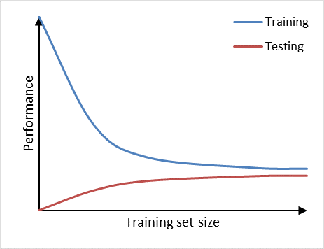
Figure 3. Prediction model suffering from high bias.

Usage

Use the OHDSI tool ecosystem to generate a population and plpData object. Alternatively, you can make use of the data simulator. The following code snippet creates a population of 12000 patients.

set.seed(1234)
data(plpDataSimulationProfile)
sampleSize <- 12000
plpData <- simulatePlpData(
  plpDataSimulationProfile,
  n = sampleSize
)

population <- createStudyPopulation(
  plpData,
  outcomeId = 2,
  binary = TRUE,
  firstExposureOnly = FALSE,
  washoutPeriod = 0,
  removeSubjectsWithPriorOutcome = FALSE,
  priorOutcomeLookback = 99999,
  requireTimeAtRisk = FALSE,
  minTimeAtRisk = 0,
  riskWindowStart = 0,
  addExposureDaysToStart = FALSE,
  riskWindowEnd = 365,
  addExposureDaysToEnd = FALSE,
  verbosity = futile.logger::INFO
)

Specify the prediction algorithm to be used.

# Use LASSO logistic regression
modelSettings <- setLassoLogisticRegression()

Specify a test fraction and a sequence of training set fractions.

testFraction <- 0.2
trainFractions <- seq(0.1, 0.8, 0.1)

Specify the test split to be used.

# Use a split by person, alterantively a time split is possible
testSplit <- 'person'

Create the learning curve object.

learningCurve <- createLearningCurve(
  population,
  plpData = plpData,
  modelSettings = modelSettings,
  testFraction = testFraction,
  trainFractions = trainFractions,
  splitSeed = 1000,
  saveModel = FALSE,
  timeStamp = FALSE
)

Plot the learning curve object (Figure 4). Specify one of the available metrics: AUROC, AUPRC, sBrier.

plotLearningCurve(
  learningCurve,
  metric='AUROC',
  plotTitle = 'Learning Curve',
  plotSubtitle = 'AUROC performance'
)

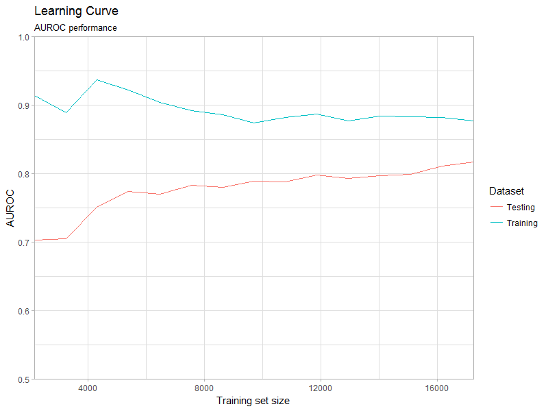
Figure 4. Learning curve plot.

Parallel processing

The learning curve object can be created in parallel, which can reduce computation time significantly. Currently this functionality is only available for LASSO logistic regression. Depending on the number of parallel workers it may require a significant amount of memory. We advise to use the parallelized learning curve function for parameter search and exploratory data analysis. Logging and saving functionality is unavailable.

Use the parallelized version of the learning curve function to create the learning curve object in parallel. R will find the number of available processing cores automatically and register the required parallel backend.

learningCurvePar <- createLearningCurvePar(
  population,
  plpData =  plpData,
  modelSettings = modelSettings,
  testSplit = testSplit,
  testFraction = testFraction,
  trainFractions = trainFractions,
  splitSeed = 1000
)