4  Building analytic pipelines for a data model

In the previous chapters, we’ve seen that after connecting to a database, we can create references to the various tables we’re interested in and write custom analytic code to query them. However, if we are working with the same database over and over again, we might want to build some tooling for tasks we often perform.

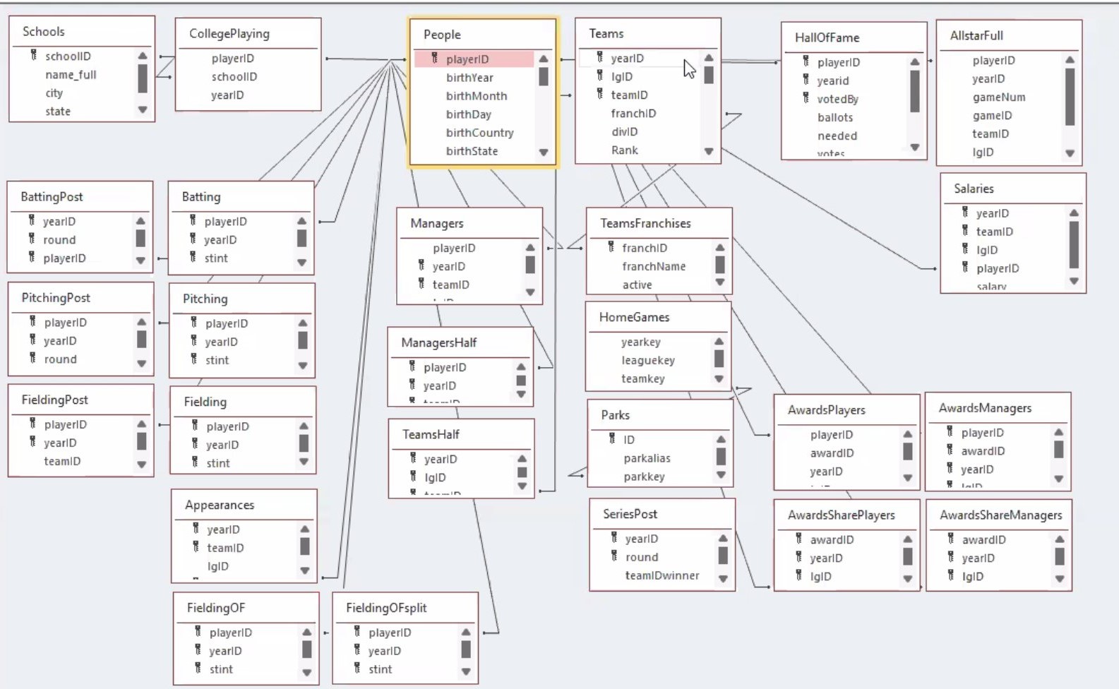
To see how we can develop a data model with associated methods and functions, we will use the Lahman baseball data. The data is stored across various related tables.

Figure 4.1: Lahman’s Baseball Dabatase schema from https://cdalzell.github.io/Lahman/.

4.1 Defining a data model

library(duckdb)
library(dplyr)
library(tidyr)
library(purrr)
library(cli)
library(dbplyr)
library(Lahman)

con <- dbConnect(drv = duckdb())
copy_lahman(con = con)

Notecopy_lahman

The copy_lahman() function inserts all the different tables in the connection. It works in the same way as we have done before with the for loop and the dbWriteTable() function.

See that there are 28 new tables inserted in our DuckDB database:

dbListTables(conn = con)

 [1] "AllstarFull"         "Appearances"         "AwardsManagers"     
 [4] "AwardsPlayers"       "AwardsShareManagers" "AwardsSharePlayers" 
 [7] "Batting"             "BattingPost"         "CollegePlaying"     
[10] "Fielding"            "FieldingOF"          "FieldingOFsplit"    
[13] "FieldingPost"        "HallOfFame"          "HomeGames"          
[16] "LahmanData"          "Managers"            "ManagersHalf"       
[19] "Parks"               "People"              "Pitching"           
[22] "PitchingPost"        "Salaries"            "Schools"            
[25] "SeriesPost"          "Teams"               "TeamsFranchises"    
[28] "TeamsHalf"          

Instead of manually creating references for each one of the tables (so we can access them easily), we will write a function to create a single reference to the Lahman data.

lahmanFromCon <- function(con) {
  lahmanRef <- set_names(c(
    "AllstarFull", "Appearances", "AwardsManagers", "AwardsPlayers", "AwardsManagers",
    "AwardsShareManagers", "Batting", "BattingPost", "CollegePlaying", "Fielding",
    "FieldingOF", "FieldingOFsplit", "FieldingPost", "HallOfFame", "HomeGames",
    "LahmanData", "Managers", "ManagersHalf", "Parks", "People", "Pitching",
    "PitchingPost", "Salaries", "Schools", "SeriesPost", "Teams", "TeamsFranchises",
    "TeamsHalf"
  ))
  
  lahmanRef <- map(lahmanRef, \(x) tbl(src = con, from = x))
  
  class(lahmanRef) <- c("lahman_ref", class(lahmanRef))
  return(lahmanRef)
}

With this function we can now easily get references to all our Lahman tables in one go using our lahmanFromCon() function.

lahman <- lahmanFromCon(con = con)

lahman$People |>
  glimpse()

Rows: ??
Columns: 26
Database: DuckDB 1.4.1 [unknown@Linux 6.11.0-1018-azure:R 4.4.1/:memory:]
$ playerID     <chr> "aardsda01", "aaronha01", "aaronto01", "aasedo01", "abada…
$ birthYear    <int> 1981, 1934, 1939, 1954, 1972, 1985, 1850, 1877, 1869, 186…
$ birthMonth   <int> 12, 2, 8, 9, 8, 12, 11, 4, 11, 10, 6, 9, 3, 10, 2, 8, 9, …
$ birthDay     <int> 27, 5, 5, 8, 25, 17, 4, 15, 11, 14, 1, 20, 16, 22, 16, 17…
$ birthCity    <chr> "Denver", "Mobile", "Mobile", "Orange", "Palm Beach", "La…
$ birthCountry <chr> "USA", "USA", "USA", "USA", "USA", "D.R.", "USA", "USA", …
$ birthState   <chr> "CO", "AL", "AL", "CA", "FL", "La Romana", "PA", "PA", "V…
$ deathYear    <int> NA, 2021, 1984, NA, NA, NA, 1905, 1957, 1962, 1926, NA, N…
$ deathMonth   <int> NA, 1, 8, NA, NA, NA, 5, 1, 6, 4, NA, NA, 2, 6, NA, NA, N…
$ deathDay     <int> NA, 22, 16, NA, NA, NA, 17, 6, 11, 27, NA, NA, 13, 11, NA…
$ deathCountry <chr> NA, "USA", "USA", NA, NA, NA, "USA", "USA", "USA", "USA",…
$ deathState   <chr> NA, "GA", "GA", NA, NA, NA, "NJ", "FL", "VT", "CA", NA, N…
$ deathCity    <chr> NA, "Atlanta", "Atlanta", NA, NA, NA, "Pemberton", "Fort …
$ nameFirst    <chr> "David", "Hank", "Tommie", "Don", "Andy", "Fernando", "Jo…
$ nameLast     <chr> "Aardsma", "Aaron", "Aaron", "Aase", "Abad", "Abad", "Aba…
$ nameGiven    <chr> "David Allan", "Henry Louis", "Tommie Lee", "Donald Willi…
$ weight       <int> 215, 180, 190, 190, 184, 235, 192, 170, 175, 169, 192, 22…
$ height       <int> 75, 72, 75, 75, 73, 74, 72, 71, 71, 68, 72, 74, 71, 70, 7…
$ bats         <fct> R, R, R, R, L, L, R, R, R, L, L, R, R, R, R, R, L, R, L, …
$ throws       <fct> R, R, R, R, L, L, R, R, R, L, L, R, R, R, R, L, L, R, L, …
$ debut        <chr> "2004-04-06", "1954-04-13", "1962-04-10", "1977-07-26", "…
$ bbrefID      <chr> "aardsda01", "aaronha01", "aaronto01", "aasedo01", "abada…
$ finalGame    <chr> "2015-08-23", "1976-10-03", "1971-09-26", "1990-10-03", "…
$ retroID      <chr> "aardd001", "aaroh101", "aarot101", "aased001", "abada001…
$ deathDate    <date> NA, 2021-01-22, 1984-08-16, NA, NA, NA, 1905-05-17, 1957…
$ birthDate    <date> 1981-12-27, 1934-02-05, 1939-08-05, 1954-09-08, 1972-08-…

NoteThe dm package

In this chapter we will be creating a bespoke data model for our database. This approach can be further extended using the dm package, which also provides various helpful functions for creating a data model and working with it.

Similar to above, we can use dm() to create a single object to access our database tables.

library(dm)
lahman_dm <- dm(batting = tbl(con, "Batting"), people = tbl(con, "People"))
lahman_dm

── Table source ────────────────────────────────────────────────────────────────
src:  DuckDB 1.4.1 [unknown@Linux 6.11.0-1018-azure:R 4.4.1/:memory:]
── Metadata ────────────────────────────────────────────────────────────────────
Tables: `batting`, `people`
Columns: 48
Primary keys: 0
Foreign keys: 0

Using this approach, we can make use of various utility functions. For example here we specify primary and foreign keys and then check that the key constraints are satisfied.

lahman_dm <- lahman_dm |>
  dm_add_pk(table = "people", columns = "playerID") |>
  dm_add_fk(table = "batting", columns = "playerID", ref_table = "people") 

lahman_dm

── Table source ────────────────────────────────────────────────────────────────
src:  DuckDB 1.4.1 [unknown@Linux 6.11.0-1018-azure:R 4.4.1/:memory:]
── Metadata ────────────────────────────────────────────────────────────────────
Tables: `batting`, `people`
Columns: 48
Primary keys: 1
Foreign keys: 1

dm_examine_constraints(.dm = lahman_dm)

ℹ All constraints satisfied.

For more information on the dm package see https://dm.cynkra.com/index.html

4.2 Creating functions for the data model

Given that we know the structure of the data, we can build a set of functions tailored to the Lahman data model to simplify data analyses.

Let’s start by creating a simple function that returns the teams each player has played for. We can see that the code we use follows on from the last couple of chapters.

getTeams <- function(lahman, name = "Barry Bonds") {
  lahman$Batting |>
    inner_join(
      lahman$People |>
        mutate(full_name = paste0(nameFirst, " ", nameLast)) |>
        filter(full_name %in% name) |>
        select("playerID"),
      by = "playerID"
    ) |>
    distinct(teamID, yearID) |>
    left_join(
      lahman$Teams, 
      by = c("teamID", "yearID")) |>
    distinct(name)
}

Now we can easily get which teams a player has represented. We can see how changing the player name changes the SQL that is run behind the scenes.

getTeams(lahman = lahman, name = "Babe Ruth")

# Source:   SQL [?? x 1]
# Database: DuckDB 1.4.1 [unknown@Linux 6.11.0-1018-azure:R 4.4.1/:memory:]
  name            
  <chr>           
1 Boston Braves   
2 Boston Red Sox  
3 New York Yankees

NoteShow query

<SQL>
SELECT DISTINCT q01.*
FROM (
  SELECT "name"
  FROM (
    SELECT DISTINCT q01.*
    FROM (
      SELECT teamID, yearID
      FROM Batting
      INNER JOIN (
        SELECT playerID
        FROM (
          SELECT People.*, CONCAT_WS('', nameFirst, ' ', nameLast) AS full_name
          FROM People
        ) q01
        WHERE (full_name IN ('Babe Ruth'))
      ) RHS
        ON (Batting.playerID = RHS.playerID)
    ) q01
  ) LHS
  LEFT JOIN Teams
    ON (LHS.teamID = Teams.teamID AND LHS.yearID = Teams.yearID)
) q01

getTeams(lahman = lahman, name = "Barry Bonds")

# Source:   SQL [?? x 1]
# Database: DuckDB 1.4.1 [unknown@Linux 6.11.0-1018-azure:R 4.4.1/:memory:]
  name                
  <chr>               
1 Pittsburgh Pirates  
2 San Francisco Giants

NoteShow query

<SQL>
SELECT DISTINCT q01.*
FROM (
  SELECT "name"
  FROM (
    SELECT DISTINCT q01.*
    FROM (
      SELECT teamID, yearID
      FROM Batting
      INNER JOIN (
        SELECT playerID
        FROM (
          SELECT People.*, CONCAT_WS('', nameFirst, ' ', nameLast) AS full_name
          FROM People
        ) q01
        WHERE (full_name IN ('Barry Bonds'))
      ) RHS
        ON (Batting.playerID = RHS.playerID)
    ) q01
  ) LHS
  LEFT JOIN Teams
    ON (LHS.teamID = Teams.teamID AND LHS.yearID = Teams.yearID)
) q01

TipChoosing the right time to collect data into R

The function collect() brings data out of the database and into R. When working with large datasets, as is often the case when interacting with a database, we typically want to keep as much computation as possible on the database side. In the case of our getTeams() function, for example, everything is done on the database side. Collecting the result will bring the result of the teams the person played for out of the database. In this case, we could also use pull() to get our result out as a vector rather than a data frame.

getTeams(lahman = lahman, name = "Barry Bonds") |>
  collect()

# A tibble: 2 × 1
  name                
  <chr>               
1 San Francisco Giants
2 Pittsburgh Pirates  

getTeams(lahman = lahman, name = "Barry Bonds") |>
  pull()

[1] "San Francisco Giants" "Pittsburgh Pirates"  

However, in other cases we may need to collect the data to perform analyses that can not be done in SQL. This might be the case for plotting or for other analytic steps(i.e., fitting statistical models). In such cases, it is important to only bring out the data that we need (as our local computer will typically have far less memory available than the database system).

Similarly, we can make a function to add a player’s year of birth to another Lahman table.

addBirthCountry <- function(x){
  x |> 
    left_join(
      lahman$People |> 
        select("playerID", "birthCountry"),
      by = "playerID"
    )
}

lahman$Batting |>
  addBirthCountry()

# Source:   SQL [?? x 23]
# Database: DuckDB 1.4.1 [unknown@Linux 6.11.0-1018-azure:R 4.4.1/:memory:]
   playerID  yearID stint teamID lgID      G    AB     R     H   X2B   X3B    HR
   <chr>      <int> <int> <fct>  <fct> <int> <int> <int> <int> <int> <int> <int>
 1 aardsda01   2004     1 SFN    NL       11     0     0     0     0     0     0
 2 aardsda01   2006     1 CHN    NL       45     2     0     0     0     0     0
 3 aardsda01   2007     1 CHA    AL       25     0     0     0     0     0     0
 4 aardsda01   2008     1 BOS    AL       47     1     0     0     0     0     0
 5 aardsda01   2009     1 SEA    AL       73     0     0     0     0     0     0
 6 aardsda01   2010     1 SEA    AL       53     0     0     0     0     0     0
 7 aardsda01   2012     1 NYA    AL        1     0     0     0     0     0     0
 8 aardsda01   2013     1 NYN    NL       43     0     0     0     0     0     0
 9 aardsda01   2015     1 ATL    NL       33     1     0     0     0     0     0
10 aaronha01   1954     1 ML1    NL      122   468    58   131    27     6    13
# ℹ more rows
# ℹ 11 more variables: RBI <int>, SB <int>, CS <int>, BB <int>, SO <int>,
#   IBB <int>, HBP <int>, SH <int>, SF <int>, GIDP <int>, birthCountry <chr>

NoteShow query

<SQL>
SELECT Batting.*, birthCountry
FROM Batting
LEFT JOIN People
  ON (Batting.playerID = People.playerID)

lahman$Pitching |>
  addBirthCountry()

# Source:   SQL [?? x 31]
# Database: DuckDB 1.4.1 [unknown@Linux 6.11.0-1018-azure:R 4.4.1/:memory:]
   playerID  yearID stint teamID lgID      W     L     G    GS    CG   SHO    SV
   <chr>      <int> <int> <fct>  <fct> <int> <int> <int> <int> <int> <int> <int>
 1 aardsda01   2004     1 SFN    NL        1     0    11     0     0     0     0
 2 aardsda01   2006     1 CHN    NL        3     0    45     0     0     0     0
 3 aardsda01   2007     1 CHA    AL        2     1    25     0     0     0     0
 4 aardsda01   2008     1 BOS    AL        4     2    47     0     0     0     0
 5 aardsda01   2009     1 SEA    AL        3     6    73     0     0     0    38
 6 aardsda01   2010     1 SEA    AL        0     6    53     0     0     0    31
 7 aardsda01   2012     1 NYA    AL        0     0     1     0     0     0     0
 8 aardsda01   2013     1 NYN    NL        2     2    43     0     0     0     0
 9 aardsda01   2015     1 ATL    NL        1     1    33     0     0     0     0
10 aasedo01    1977     1 BOS    AL        6     2    13    13     4     2     0
# ℹ more rows
# ℹ 19 more variables: IPouts <int>, H <int>, ER <int>, HR <int>, BB <int>,
#   SO <int>, BAOpp <dbl>, ERA <dbl>, IBB <int>, WP <int>, HBP <int>, BK <int>,
#   BFP <int>, GF <int>, R <int>, SH <int>, SF <int>, GIDP <int>,
#   birthCountry <chr>

NoteShow query

<SQL>
SELECT Pitching.*, birthCountry
FROM Pitching
LEFT JOIN People
  ON (Pitching.playerID = People.playerID)

We can then use our addBirthCountry() function as part of a larger query to summarise and plot the proportion of players from each country over time (based on their presence in the batting table).

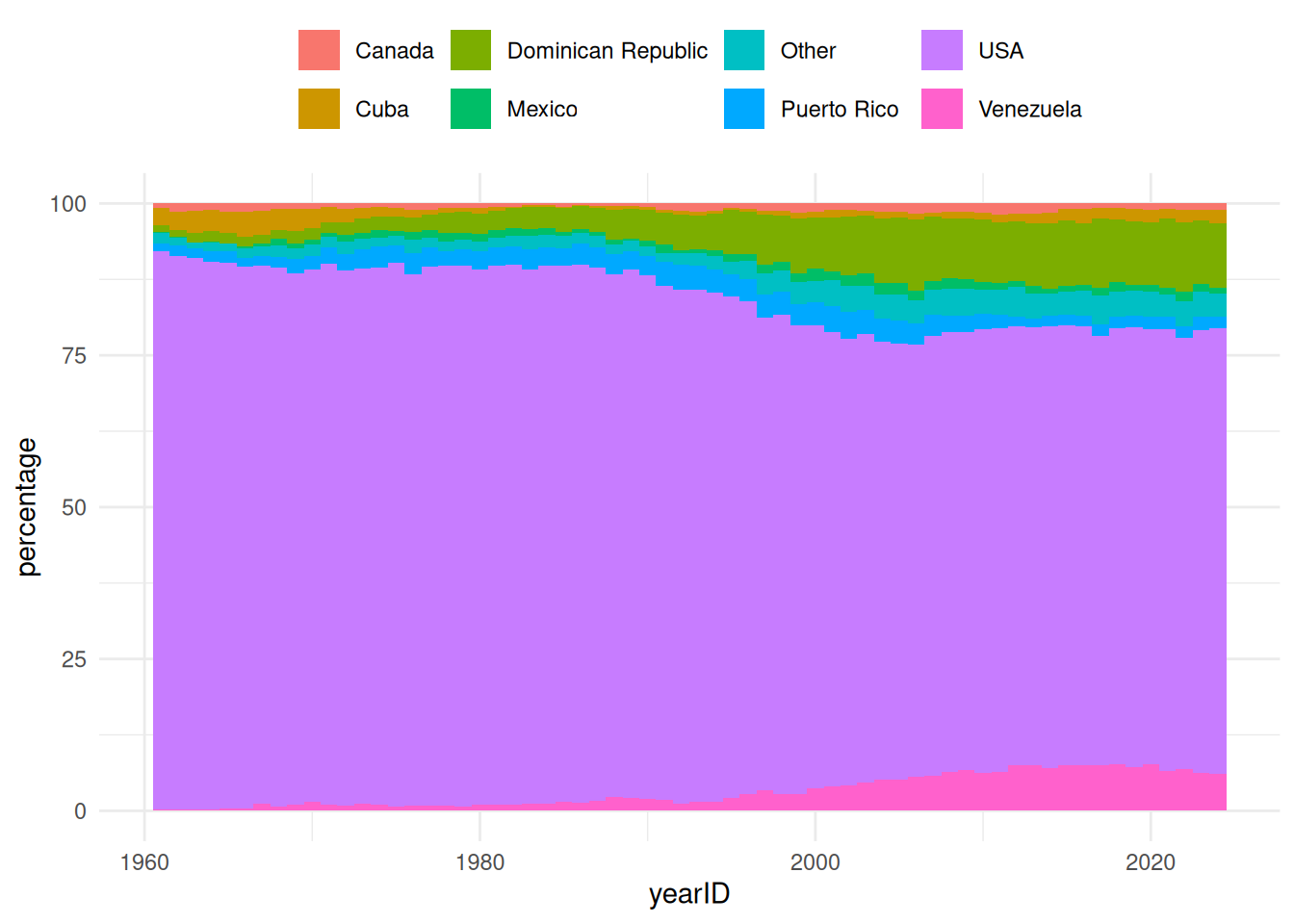
plot_data <- lahman$Batting |>
  select("playerID", "yearID") |> 
  addBirthCountry() |>
  filter(yearID > 1960) |> 
  mutate(birthCountry = case_when(
    birthCountry == "USA" ~ "USA",
    birthCountry == "D.R." ~ "Dominican Republic",
    birthCountry == "Venezuela" ~ "Venezuela",
    birthCountry == "P.R." ~ "Puerto Rico ",
    birthCountry == "Cuba" ~ "Cuba",
    birthCountry == "CAN" ~ "Canada",
    birthCountry == "Mexico" ~ "Mexico",
    .default = "Other"
  )) |> 
  group_by(yearID, birthCountry) |>
  summarise(n = n(), .groups = "drop") |> 
  group_by(yearID) |>
  mutate(percentage = n / sum(n) * 100) |> 
  ungroup() |> 
  collect()

NoteShow query

<SQL>
SELECT q01.*, (n / SUM(n) OVER (PARTITION BY yearID)) * 100.0 AS percentage
FROM (
  SELECT yearID, birthCountry, COUNT(*) AS n
  FROM (
    SELECT
      playerID,
      yearID,
      CASE
WHEN (birthCountry = 'USA') THEN 'USA'
WHEN (birthCountry = 'D.R.') THEN 'Dominican Republic'
WHEN (birthCountry = 'Venezuela') THEN 'Venezuela'
WHEN (birthCountry = 'P.R.') THEN 'Puerto Rico '
WHEN (birthCountry = 'Cuba') THEN 'Cuba'
WHEN (birthCountry = 'CAN') THEN 'Canada'
WHEN (birthCountry = 'Mexico') THEN 'Mexico'
ELSE 'Other'
END AS birthCountry
    FROM (
      SELECT Batting.playerID AS playerID, yearID, birthCountry
      FROM Batting
      LEFT JOIN People
        ON (Batting.playerID = People.playerID)
    ) q01
    WHERE (yearID > 1960.0)
  ) q01
  GROUP BY yearID, birthCountry
) q01

library(ggplot2)
plot_data |> 
  ggplot() +
  geom_col(
    mapping = aes(yearID, percentage, fill = birthCountry), 
    width = 1
  ) + 
  theme_minimal() + 
  theme(
    legend.title = element_blank(), 
    legend.position = "top"
  )

NoteDefining methods for the data model

As part of our lahmanFromCon() function, our data model object has the class “lahman_ref”. Therefore, apart from creating user-friendly functions to work with our Lahman data model, we can also define methods for this object.

class(lahman)

[1] "lahman_ref" "list"      

With this we can make some specific methods for a “lahman_ref” object. For example, we can define a print method like so:

print.lahman_ref <- function(x, ...) {
  len <- length(names(x))
  cli_h1("# Lahman reference - {len} tables")
  cli_li(paste("{.strong tables:}", paste(names(x), collapse = ", ")))
  invisible(x)
}

Now we can see a summary of our Lahman data model when we print the object.

lahman

── # Lahman reference - 28 tables ──────────────────────────────────────────────

• tables: AllstarFull, Appearances, AwardsManagers, AwardsPlayers,
AwardsManagers, AwardsShareManagers, Batting, BattingPost, CollegePlaying,
Fielding, FieldingOF, FieldingOFsplit, FieldingPost, HallOfFame, HomeGames,
LahmanData, Managers, ManagersHalf, Parks, People, Pitching, PitchingPost,
Salaries, Schools, SeriesPost, Teams, TeamsFranchises, TeamsHalf

And we can see that this print is being done by the method we defined.

library(sloop)
s3_dispatch(print(lahman))

=> print.lahman_ref
   print.list
 * print.default

4.3 Building efficient analytic pipelines

4.3.1 The risk of “clean” R code

Following on from the above approach, we might think it is a good idea to make another function addBirthYear(). We can then use it along with our addBirthCountry() to get a summarised average salary by birth country and birth year.

addBirthYear <- function(lahmanTbl){
  lahmanTbl |> 
    left_join(
      lahman$People |> 
        select("playerID", "birthYear"),
      by = "playerID"
    )
}

lahman$Salaries |> 
  addBirthCountry() |> 
  addBirthYear() |> 
  group_by(birthCountry, birthYear) |>
  summarise(average_salary = mean(salary), .groups = "drop")

# Source:   SQL [?? x 3]
# Database: DuckDB 1.4.1 [unknown@Linux 6.11.0-1018-azure:R 4.4.1/:memory:]
   birthCountry birthYear average_salary
   <chr>            <int>          <dbl>
 1 USA               1966       1761151.
 2 Venezuela         1974       4269365.
 3 D.R.              1984       2924854.
 4 Mexico            1982       1174912.
 5 Panama            1981        555833.
 6 USA               1978       3133596.
 7 P.R.              1959        297786.
 8 USA               1961        811250.
 9 USA               1990        728740.
10 USA               1950        625076.
# ℹ more rows

Although the R code looks fine, when we look at the SQL we can see that our query has two joins to the People table. One join gets information on the birth country and the other on the birth year.

NoteShow query

<SQL>
SELECT birthCountry, birthYear, AVG(salary) AS average_salary
FROM (
  SELECT
    Salaries.*,
    "People...2".birthCountry AS birthCountry,
    "People...3".birthYear AS birthYear
  FROM Salaries
  LEFT JOIN People "People...2"
    ON (Salaries.playerID = "People...2".playerID)
  LEFT JOIN People "People...3"
    ON (Salaries.playerID = "People...3".playerID)
) q01
GROUP BY birthCountry, birthYear

To improve the performance of the code, we can build a single function to get simultaneously the birth country and birth year, so only one join is done.

addCharacteristics <- function(lahmanTbl) {
  lahmanTbl |> 
    left_join(
      lahman$People |> 
        select("playerID", "birthYear", "birthCountry"),
      by = "playerID"
    )
}

lahman$Salaries |> 
  addCharacteristics() |> 
  group_by(birthCountry, birthYear) |>
  summarise(average_salary = mean(salary), .groups = "drop")

# Source:   SQL [?? x 3]
# Database: DuckDB 1.4.1 [unknown@Linux 6.11.0-1018-azure:R 4.4.1/:memory:]
   birthCountry birthYear average_salary
   <chr>            <int>          <dbl>
 1 USA               1966       1761151.
 2 Venezuela         1974       4269365.
 3 D.R.              1984       2924854.
 4 Mexico            1982       1174912.
 5 Panama            1981        555833.
 6 USA               1978       3133596.
 7 P.R.              1959        297786.
 8 USA               1961        811250.
 9 USA               1990        728740.
10 USA               1950        625076.
# ℹ more rows

NoteShow query

<SQL>
SELECT birthCountry, birthYear, AVG(salary) AS average_salary
FROM (
  SELECT Salaries.*, birthYear, birthCountry
  FROM Salaries
  LEFT JOIN People
    ON (Salaries.playerID = People.playerID)
) q01
GROUP BY birthCountry, birthYear

This query produces the same result but is simpler than the previous one, thus reducing the computational cost of the analysis. This shows the importance of being aware of the SQL code being executed when working in R with databases.

4.3.2 Piping and SQL

Piping functions has little impact on performance when using R with data in memory. However, when working with a database, the SQL generated will differ when using multiple function calls (with a separate operation specified in each) instead of multiple operations within a single function call.

For example, a single mutate function creating two new variables would generate the below SQL.

lahman$People |> 
  mutate(
    birthDatePlus1 = add_years(x = birthDate, n = 1L),
    birthDatePlus10 = add_years(x = birthDate, n = 10L)
  ) |> 
  select("playerID", "birthDatePlus1", "birthDatePlus10") |> 
  show_query()

<SQL>
SELECT
  playerID,
  DATE_ADD(birthDate, INTERVAL (1) year) AS birthDatePlus1,
  DATE_ADD(birthDate, INTERVAL (10) year) AS birthDatePlus10
FROM People

Whereas the SQL will be different if these were created using multiple mutate calls (with now one being created in a sub-query).

lahman$People |> 
  mutate(birthDatePlus1 = add_years(x = birthDate, n = 1L)) |> 
  mutate(birthDatePlus10 = add_years(x = birthDate, n = 10L)) |> 
  select("playerID", "birthDatePlus1", "birthDatePlus10") |> 
  show_query()

<SQL>
SELECT
  playerID,
  birthDatePlus1,
  DATE_ADD(birthDate, INTERVAL (10) year) AS birthDatePlus10
FROM (
  SELECT People.*, DATE_ADD(birthDate, INTERVAL (1) year) AS birthDatePlus1
  FROM People
) q01

4.3.3 Computing intermediate queries

Let’s now summarise home runs (Batting table) and strike outs (Pitching table) by college player and their birth year. We can do this like so:

players_with_college <- lahman$People |> 
  select("playerID", "birthYear") |> 
  inner_join(
    lahman$CollegePlaying |> 
      filter(!is.na(schoolID)) |> 
      distinct(playerID, schoolID),
    by = "playerID"
  )

lahman$Batting |> 
  left_join(
    players_with_college,
    by = "playerID"
  ) |> 
  group_by(schoolID, birthYear) |>
  summarise(home_runs = sum(H, na.rm = TRUE), .groups = "drop") |> 
  collect()

# A tibble: 6,205 × 3
   schoolID   birthYear home_runs
   <chr>          <int>     <dbl>
 1 gamiddl         1972         2
 2 illinoisst      1981         1
 3 lehigh          1901         1
 4 tamukvill       1978         0
 5 chicago         1874         2
 6 capalom         1963        15
 7 hawaiipac       1971       299
 8 bostonuniv      1929       135
 9 byu             1961        28
10 kentucky        1985         1
# ℹ 6,195 more rows

lahman$Pitching |> 
  left_join(
    players_with_college, 
    by = "playerID"
  ) |> 
  group_by(schoolID, birthYear) |>
  summarise(strike_outs = sum(SO, na.rm = TRUE), .groups = "drop") |> 
  collect()

# A tibble: 3,663 × 3
   schoolID   birthYear strike_outs
   <chr>          <int>       <dbl>
 1 rice            1981         340
 2 cacerri         1971         327
 3 usc             1947         275
 4 pepperdine      1969           4
 5 lsu             1978         162
 6 miamidade       1982          56
 7 upperiowa       1918          11
 8 jamesmad        1966           4
 9 flinternat      1971         133
10 ucla            1984         323
# ℹ 3,653 more rows

If we look at the SQL code we will realise that there is code duplication, because as part of each full query, we have run our players_with_college query.

NoteShow query

<SQL>
SELECT schoolID, birthYear, SUM(H) AS home_runs
FROM (
  SELECT Batting.*, birthYear, schoolID
  FROM Batting
  LEFT JOIN (
    SELECT People.playerID AS playerID, birthYear, schoolID
    FROM People
    INNER JOIN (
      SELECT DISTINCT playerID, schoolID
      FROM CollegePlaying
      WHERE (NOT((schoolID IS NULL)))
    ) RHS
      ON (People.playerID = RHS.playerID)
  ) RHS
    ON (Batting.playerID = RHS.playerID)
) q01
GROUP BY schoolID, birthYear

<SQL>
SELECT schoolID, birthYear, SUM(SO) AS strike_outs
FROM (
  SELECT Pitching.*, birthYear, schoolID
  FROM Pitching
  LEFT JOIN (
    SELECT People.playerID AS playerID, birthYear, schoolID
    FROM People
    INNER JOIN (
      SELECT DISTINCT playerID, schoolID
      FROM CollegePlaying
      WHERE (NOT((schoolID IS NULL)))
    ) RHS
      ON (People.playerID = RHS.playerID)
  ) RHS
    ON (Pitching.playerID = RHS.playerID)
) q01
GROUP BY schoolID, birthYear

To avoid this, we can make use of the compute() function to force the computation of the players_with_college query to a temporary table in the database.

players_with_college <- players_with_college |> 
  compute()

Now we have a temporary table with the result of our players_with_college query, and we can use this in both of our aggregation queries.

players_with_college |> 
  show_query()

<SQL>
SELECT *
FROM dbplyr_9p8AfFYmY7

lahman$Batting |> 
  left_join(players_with_college, by = "playerID") |> 
  group_by(schoolID, birthYear) |>
  summarise(home_runs = sum(H, na.rm = TRUE), .groups = "drop") |> 
  collect()

# A tibble: 6,205 × 3
   schoolID  birthYear home_runs
   <chr>         <int>     <dbl>
 1 kentucky       1972       157
 2 longbeach      1968        19
 3 elon           1921         1
 4 lehigh         1901         1
 5 ucla           1952       306
 6 usc            1947        11
 7 tamukvill      1978         0
 8 stanford       1972        55
 9 lsu            1927      1832
10 wake           1915        72
# ℹ 6,195 more rows

lahman$Pitching |> 
  left_join(players_with_college, by = "playerID") |> 
  group_by(schoolID, birthYear) |>
  summarise(strike_outs = sum(SO, na.rm = TRUE), .groups = "drop") |> 
  collect()

# A tibble: 3,663 × 3
   schoolID   birthYear strike_outs
   <chr>          <int>       <dbl>
 1 vermont         1869         161
 2 michigan        1967         888
 3 nmstate         1968          98
 4 cacerri         1971         327
 5 byu             1961        1030
 6 pepperdine      1969           4
 7 lsu             1978         162
 8 miamidade       1982          56
 9 stanford        1961           0
10 incante         1893         526
# ℹ 3,653 more rows

NoteShow query

<SQL>
SELECT schoolID, birthYear, SUM(H) AS home_runs
FROM (
  SELECT Batting.*, birthYear, schoolID
  FROM Batting
  LEFT JOIN dbplyr_9p8AfFYmY7
    ON (Batting.playerID = dbplyr_9p8AfFYmY7.playerID)
) q01
GROUP BY schoolID, birthYear

<SQL>
SELECT schoolID, birthYear, SUM(SO) AS strike_outs
FROM (
  SELECT Pitching.*, birthYear, schoolID
  FROM Pitching
  LEFT JOIN dbplyr_9p8AfFYmY7
    ON (Pitching.playerID = dbplyr_9p8AfFYmY7.playerID)
) q01
GROUP BY schoolID, birthYear

In this example, the SQL code of the intermediate table, players_with_college, was quite simple. However, in some cases, the SQL associated code can become very complicated and unmanageable, resulting with inefficient code. Therefore, although we do not want to overuse computation of intermediate queries, it is often useful when creating our analytic pipelines.

NoteIndexes

Some SQL dialects use indexes for more efficient ‘joins’ performance. Briefly speaking, indexes store the location of the different values of a column. Every time that you create a new table with compute(), the indexes will not be carried over. Hence, if you want your new table to keep some indexes, you will have to add them manually. That is why sometimes it will not be more efficient to add a compute() in between, because the new table generated will not have the indexes that make your query to be executed faster.

4.4 Disconnecting from the database

Now that we have reached the end of this example, we can close our connection to the database.

dbDisconnect(conn = con)