Single studies using the SelfControlledCaseSeries package

Introduction

This vignette describes how you can use the SelfControlledCaseSeries package to perform a single Self-Controlled Case Series (SCCS) study. We will walk through all the steps needed to perform an exemplar study, and we have selected the well-studied topic of the effect of aspirin on epistaxis.

Terminology

The following terms are used consistently throughout the package:

Case: a period of continuous observation of a person containing one or more outcomes. One person can contribute to multiple cases, for example when the person has multiple observation periods.
Observation period: the time when a person is observed in the database, e.g. the time when enrolled in an insurance plan.
Nesting cohort: a cohort defining when persons are eligible to be included as cases. This is typically the indication of the drug. For example, if the drug treats diabetes, we may want to nest the analysis in the time when people have diabetes to avoid (time-varying) confounding by indication.
Study period: a period of calendar time when persons are eligible to be included as cases. For example, a study period could be January 1, 2020, onward. Unlike nesting cohorts, which could specify different time periods per person, a study period applies to all persons.
Naive period: the first part of a person’s observation period (e.g. the first 180 days). This is typically removed from the SCCS model to avoid exposure and incident outcome misclassification. For example, if we observe the outcome on the second day of a person’s observation period, we do not know whether the outcome is a new one or just a follow-up for an old one, and whether the patient may have started the exposure just prior to observation start without us knowing about it.
Study population: the set of cases having a specific outcome, that meet certain criteria, such as the naive period and age restrictions.
Era: a data element extracted from the database denoting a time period for a patient (a case). This can be a cohort, but also a drug era.
SCCS data: a data object containing information on cases, observation periods, nesting cohorts, and eras.
Covariate: a time-varying variable used as a predictor for the outcome in the SCCS model. These include splines and era covariates.
Era covariate: a covariate derived from an era. Multiple covariates can be derived from a single era (e.g. a covariate for when on a drug, and a covariate for the pre-exposure time prior to the drug). One covariate can be derived from multiple eras (e.g. one covariate can represent a class of drugs).
SCCS interval data: data of cases chopped into intervals during which all covariates have a constant value. For splines (e.g for season), the effect is assumed to be constant within each calendar month.
SCCS model: a Poisson regression of SCCS interval data, condition on the observation period.

Installation instructions

Before installing the SelfControlledCaseSeries package make sure you have Java available. For Windows users, RTools is also necessary. See these instructions for properly configuring your R environment.

The SelfControlledCaseSeries package is maintained in a Github repository, and can be downloaded and installed from within R using the remotes package:

install.packages("remotes")
library(remotes)
install_github("ohdsi/SelfControlledCaseSeries")

Once installed, you can type library(SelfControlledCaseSeries) to load the package.

Overview

In the SelfControlledCaseSeries package a study requires at least three steps:

Loading the necessary data from the database.
Transforming the data into a format suitable for an SCCS study. This step can be broken down in multiple tasks:

Defining a study population, people having a specific outcome, with possible further restrictions such as age.
Creating covariates based on the variables extracted from the database, such as defining risk windows based on exposures.
Transforming the data into non-overlapping time intervals, with information on the various covariates and outcomes per interval.

Fitting the model using conditional Poisson regression.

In the following sections these steps will be demonstrated for increasingly complex studies.

Studies with a single drug

Configuring the connection to the server

We need to tell R how to connect to the server where the data are. SelfControlledCaseSeries uses the DatabaseConnector package, which provides the createConnectionDetails function. Type ?createConnectionDetails for the specific settings required for the various database management systems (DBMS). For example, one might connect to a PostgreSQL database using this code:

connectionDetails <- createConnectionDetails(dbms = "postgresql", 
                                             server = "localhost/ohdsi", 
                                             user = "joe", 
                                             password = "supersecret")

cdmDatabaseSchema <- "my_cdm_data"
cohortDatabaseSchema <- "my_results"
cohortTable <- "my_cohorts"
options(sqlRenderTempEmulationSchema = NULL)

The last lines define the cdmDatabaseSchema, cohortDatabaseSchema, and cohortTable variables. We’ll use these later to tell R where the data in CDM format live, where we have stored our cohorts of interest, and what version CDM is used. Note that for Microsoft SQL Server, databaseSchemas need to specify both the database and the schema, so for example cdmDatabaseSchema <- "my_cdm_data.dbo". For database platforms that do not support temp tables, such as Oracle, it is also necessary to provide a schema where the user has write access that can be used to emulate temp tables. PostgreSQL supports temp tables, so we can set options(sqlRenderTempEmulationSchema = NULL) (or not set the sqlRenderTempEmulationSchema at all.)

Preparing the exposure and outcome of interest

We need to define the exposure and outcome for our study. For the exposure, we will directly use the drug_era table in the CDM. For the outcome we can use the OHDSI PhenotypeLibrary package to retrieve a community-approved definition of epistaxis:

epistaxis <- 356
cohortDefinitionSet <- PhenotypeLibrary::getPlCohortDefinitionSet(epistaxis)

We can use the CohortGenerator package to instantiate this cohort:

connection <- DatabaseConnector::connect(connectionDetails)
cohortTableNames <- CohortGenerator::getCohortTableNames(cohortTable)
CohortGenerator::createCohortTables(connection = connection,
                                    cohortDatabaseSchema = cohortDatabaseSchema,
                                    cohortTableNames = cohortTableNames)
counts <- CohortGenerator::generateCohortSet(connection = connection,
                                             cdmDatabaseSchema = cdmDatabaseSchema,
                                             cohortDatabaseSchema = cohortDatabaseSchema,
                                             cohortTableNames = cohortTableNames,
                                             cohortDefinitionSet = cohortDefinitionSet)
DatabaseConnector::disconnect(connection)

Extracting the data from the server

Now we can tell SelfControlledCaseSeries to extract all necessary data for our analysis:

aspirin <- 1112807

sccsData <- getDbSccsData(
  connectionDetails = connectionDetails,
  cdmDatabaseSchema = cdmDatabaseSchema,
  outcomeDatabaseSchema = cohortDatabaseSchema,
  outcomeTable = cohortTable,
  outcomeIds = epistaxis,
  exposureDatabaseSchema = cdmDatabaseSchema,
  exposureTable = "drug_era",
  getDbSccsDataArgs = createGetDbSccsDataArgs(
    studyStartDates = "20100101",
    studyEndDates = "21000101",
    maxCasesPerOutcome = 100000,
    exposureIds = aspirin
  )
)
sccsData

## # SccsData object
## 
## Exposure cohort ID(s): 1112807
## Outcome cohort ID(s): 356
## 
## Inherits from Andromeda:
## # Andromeda object
## # Physical location:  E:\andromedaTemp\file2fb04712e5e.duckdb
## 
## Tables:
## $cases (observationPeriodId, caseId, personId, noninformativeEndCensor, observationPeriodStartDate, startDay, endDay, ageAtObsStart, genderConceptId)
## $eraRef (eraType, eraId, eraName, minObservedDate, maxObservedDate)
## $eras (eraType, caseId, eraId, eraValue, eraStartDay, eraEndDay)

There are many parameters, but they are all documented in the SelfControlledCaseSeries manual. In short, we are pointing the function to the table created earlier and indicating which cohort ID in that table identifies the outcome. Note that it is possible to fetch the data for multiple outcomes at once. We further point the function to the drug_era table, and specify the concept ID of our exposure of interest: aspirin. Again, note that it is also possible to fetch data for multiple drugs at once. In fact, when we do not specify any exposure IDs the function will retrieve the data for all the drugs found in the drug_era table.

All data about the patients, outcomes and exposures are extracted from the server and stored in the sccsData object. This object uses the Andromeda package to store information in a way that ensures R does not run out of memory, even when the data are large.

We can use the generic summary() function to view some more information of the data we extracted:

summary(sccsData)

## SccsData object summary
## 
## Exposure cohort ID(s): 1112807
## Outcome cohort ID(s): 356
## 
## Outcome counts:
##     Outcome Subjects Outcome Events Outcome Observation Periods
## 356            99202         160949                       1e+05
## 
## Eras:
## Number of era types: 2
## Number of eras: 169627

Saving the data to file

Creating the sccsData file can take considerable computing time, and it is probably a good idea to save it for future sessions. Because sccsData uses Andromeda, we cannot use R’s regular save function. Instead, we’ll have to use the saveSccsData() function:

saveSccsData(sccsData, "sccsData.zip")

We can use the loadSccsData() function to load the data in a future session.

Creating the study population

From the data fetched from the server we can now define the population we wish to study. If we retrieved data for multiple outcomes, we should now select only one, and possibly impose further restrictions:

studyPop <- createStudyPopulation(
  sccsData = sccsData,
  outcomeId = epistaxis,
  createStudyPopulationArgs = createCreateStudyPopulationArgs(
    firstOutcomeOnly = FALSE,
    naivePeriod = 180
  )
)

Here we specify we wish to study the outcome with the ID stored in epistaxis. Since this was the only outcome for which we fetched the data, we could also have skipped this argument. We furthermore specify that the first 180 days of observation of every person, the so-called ‘naive period’, will be excluded from the analysis. Note that data in the naive period will be used to determine exposure status at the start of follow-up (after the end of the naive period). We also specify we will use all occurrences of the outcome, not just the first one per person.

We can find out how many people (if any) were removed by any restrictions we imposed:

getAttritionTable(studyPop)

##   outcomeId outcomeSubjects outcomeEvents outcomeObsPeriods observedDays
## 1       356          325890        507256            331800   1211954076
## 2       356          207698        323114            211321    573067241
## 3       356           99202        160949            100000    285343718
## 4       356           87836        135825             88453    240007225
##                       description
## 1         All outcome occurrences
## 2     Outcomes in study period(s)
## 3                   Random sample
## 4 Requiring 180 days naive period

Defining a simple model

Next, we can use the data to define a simple model to fit:

covarAspirin <- createEraCovariateSettings(
  label = "Exposure of interest",
  includeEraIds = aspirin,
  start = 0,
  end = 0,
  endAnchor = "era end"
)

sccsIntervalData <- createSccsIntervalData(
  studyPopulation = studyPop,
  sccsData,
  createSccsIntervalDataArgs =  createCreateSccsIntervalDataArgs(
    eraCovariateSettings = covarAspirin
  )
)

summary(sccsIntervalData)

## SccsIntervalData object summary
## 
## Outcome cohort ID: 356
## 
## Number of cases (observation periods): 88451
## Number of eras (spans of time): 180752
## Number of outcomes: 135823
## Number of covariates: 2
## Number of non-zero covariate values: 93011

In this example, we use the createEraCovariateSettings() function to define a single covariate: exposure to aspirin. We specify that the risk window is from start of exposure to the end by setting start and end to 0, and defining the anchor for the end to be the era end, which for drug eras is the end of exposure.

We then use the covariate definition in the createSccsIntervalData() function to generate the sccsIntervalData. This represents the data in non-overlapping time intervals, with information on the various covariates and outcomes per interval.

Model fitting

The fitSccsModel function is used to fit the model:

model <- fitSccsModel(
  sccsIntervalData = sccsIntervalData,
  fitSccsModelArgs = createFitSccsModelArgs()
)

We can inspect the resulting model:

model

## SccsModel object
## 
## Outcome ID: 356
## 
## Outcome count:
##     outcomeSubjects outcomeEvents outcomeObsPeriods observedDays
## 356           87834        135823             88451    148669525
## 
## Estimates:
## # A tibble: 2 × 7
##   Name                         ID Estimate LB95CI UB95CI  LogRr SeLogRr
##   <chr>                     <dbl>    <dbl>  <dbl>  <dbl>  <dbl>   <dbl>
## 1 End of observation period    99     1.05   1.01   1.08 0.0441  0.0166
## 2 Exposure of interest       1000     1.38   1.27   1.51 0.324   0.0439

This tells us what the estimated relative risk (the incidence rate ratio) is during exposure to aspirin compared to non-exposed time.

Adding a pre-exposure window

One key assumption of the SCCS design is that the outcome does not change the subsequent probability of exposure. In this case, this assumption may be violated, because doctors may hesitate to prescribe aspirin to someone who is prone to bleeding. To ensure this does not affect our analysis, we must include a window prior to exposure. We can then test whether the rate of the outcome is increased or decreased during this pre-exposure window. Because the exposure hasn’t occurred yet, it cannot cause a change in risk. Any observed change must therefore be due to other, possibly confounding factors. We add a 30-day pre-exposure window:

covarPreAspirin <- createEraCovariateSettings(
  label = "Pre-exposure",
  includeEraIds = aspirin,
  start = -30,
  end = -1,
  endAnchor = "era start",
  preExposure = TRUE
)

sccsIntervalData <- createSccsIntervalData(
  studyPopulation = studyPop,
  sccsData,
  createSccsIntervalDataArgs = createCreateSccsIntervalDataArgs(
    eraCovariateSettings = list(covarAspirin, covarPreAspirin)
  )
)
model <- fitSccsModel(
  sccsIntervalData = sccsIntervalData,
  fitSccsModelArgs = createFitSccsModelArgs()
)

Here we created a new covariate definition in addition to the first one. We define the risk window to start 60 days prior to exposure, and end on the day just prior to exposure. We designate the covariate as preExposure = TRUE, meaning it will be used for the pre-exposure diagnostic evaluating the assumption that event and subsequent exposure are independent. We combine the two covariate settings in a list for the createSccsIntervalData function. Again, we can take a look at the results:

model

## SccsModel object
## 
## Outcome ID: 356
## 
## Outcome count:
##     outcomeSubjects outcomeEvents outcomeObsPeriods observedDays
## 356           87834        135823             88451    148669525
## 
## Estimates:
## # A tibble: 3 × 7
##   Name                         ID Estimate LB95CI UB95CI  LogRr SeLogRr
##   <chr>                     <dbl>    <dbl>  <dbl>  <dbl>  <dbl>   <dbl>
## 1 End of observation period    99     1.05   1.01   1.08 0.0448  0.0165
## 2 Exposure of interest       1000     1.44   1.32   1.57 0.363   0.0441
## 3 Pre-exposure               1001     1.37   1.23   1.52 0.312   0.0547

Including seasonality, and calendar time

Often both the rate of exposure and the outcome change with age, and can even depend on the season or calendar time in general (e.g. rates may be higher in 2021 compared to 2020). This may lead to confounding and may bias our estimates. To correct for this we can include age, season, and/or calendar time into the model.

For computational reasons we assume the effect of age, season, and calendar time are constant within each calendar month. We assume that the rate from one month to the next can be different, but we also assume that subsequent months have somewhat similar rates. This is implemented by using spline functions.

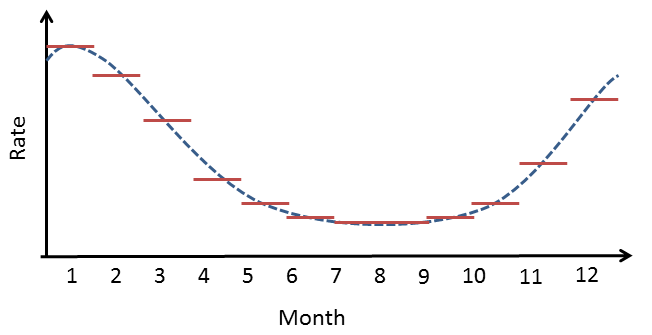Spline for seasonality Figure 1. Example of how a spline is used for seasonality: within a month, the risk attributable to seasonality is assumed to be constant, but from month to month the risks are assumed to follow a cyclic quadratic spline.

Note that by default all people that have the outcome will be used to estimate the effect of age, seasonality, and calendar time on the outcome, so not just the people exposed to the drug of interest. Adjusting for age typically only makes sense for small children, where a small difference in age can still make a big difference (remember: we are modeling the effect of age in each person by themselves, not the effect of age across persons). Since age and calendar time are often hard to fit simultaneously, it is often best to only model seasonality and calendar time, like this:

seasonalityCovariateSettings <- createSeasonalityCovariateSettings()

calendarTimeSettings <- createCalendarTimeCovariateSettings()

sccsIntervalData <- createSccsIntervalData(
  studyPopulation = studyPop,
  sccsData = sccsData,
  createSccsIntervalDataArgs = createCreateSccsIntervalDataArgs(
    eraCovariateSettings = list(covarAspirin,
                                covarPreAspirin),
    seasonalityCovariateSettings = seasonalityCovariateSettings,
    calendarTimeCovariateSettings = calendarTimeSettings
  )
)

model <- fitSccsModel(
  sccsIntervalData = sccsIntervalData,
  fitSccsModelArgs = createFitSccsModelArgs()
)

Again, we can inspect the model:

model

## SccsModel object
## 
## Outcome ID: 356
## 
## Outcome count:
##     outcomeSubjects outcomeEvents outcomeObsPeriods observedDays
## 356           13265         20611             13284     23509810
## 
## Estimates:
## # A tibble: 12 × 7
##    Name                                ID Estimate LB95CI UB95CI   LogRr SeLogRr
##    <chr>                            <dbl>    <dbl>  <dbl>  <dbl>   <dbl>   <dbl>
##  1 End of observation period           99    0.837  0.767  0.912 -0.178   0.0441
##  2 Seasonality spline component 1     200    1.37  NA     NA      0.314  NA     
##  3 Seasonality spline component 2     201    1.59  NA     NA      0.466  NA     
##  4 Seasonality spline component 3     202    1.24  NA     NA      0.218  NA     
##  5 Seasonality spline component 4     203    0.801 NA     NA     -0.222  NA     
##  6 Calendar time spline component 1   300    1.07  NA     NA      0.0656 NA     
##  7 Calendar time spline component 2   301    1.51  NA     NA      0.415  NA     
##  8 Calendar time spline component 3   302    2.14  NA     NA      0.760  NA     
##  9 Calendar time spline component 4   303    2.85  NA     NA      1.05   NA     
## 10 Calendar time spline component 5   304    3.20  NA     NA      1.16   NA     
## 11 Exposure of interest              1000    1.39   1.27   1.51   0.326   0.0442
## 12 Pre-exposure                      1001    1.33   1.19   1.47   0.282   0.0546

We see that our estimates for exposed and pre-exposure time have not changes much. We can plot the spline curves for season, and calendar time to learn more:

plotSeasonality(model)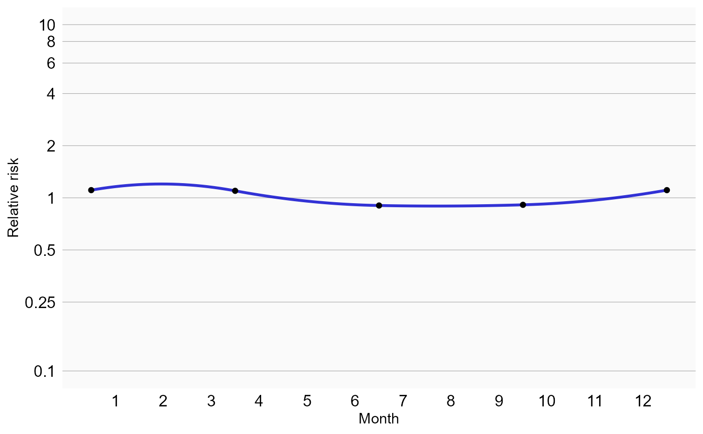

plotCalendarTimeEffect(model)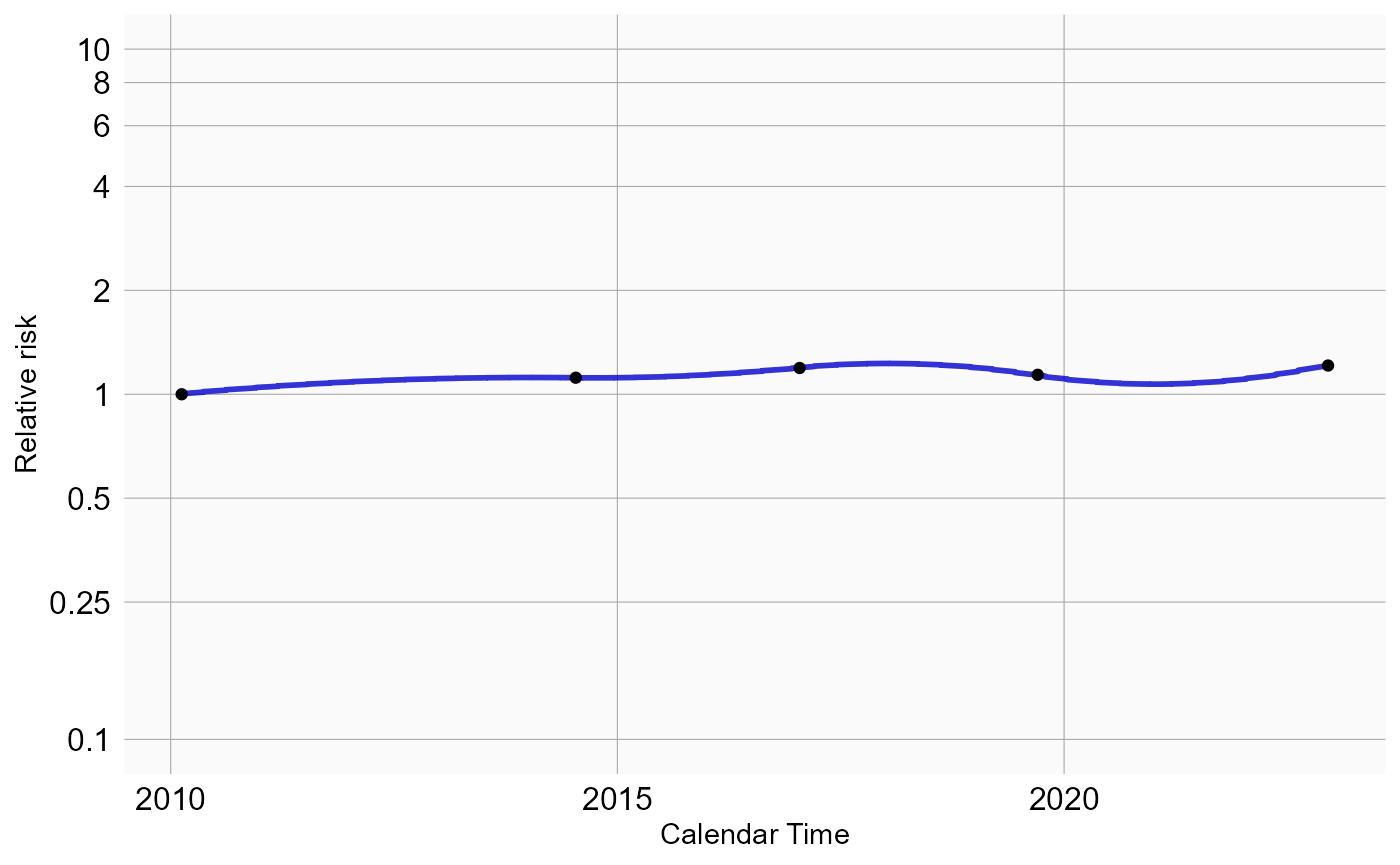

We see some effect for season: epistaxis tends to be more prevalent during winter. We should verify if our model accounts for time trends, by plotting the observed to expected rate of the outcome across time, before and after adjustment:

plotEventToCalendarTime(studyPopulation = studyPop,
                        sccsModel = model)

Here we see that after adjustment, in general, the rate of outcome appears fairly stable across time, with the exception of some months in 2020. This is what we refer to as the ‘COVID-blip’, because during the time of the COVID-19 pandemic regular healthcare was put on hold.

Removing the COVID blip

The discontinuity in the rate of the outcome during the COVID pandemic could cause bias. For this reason it is probably best to remove this time from the analysis altogether. We can achieve this by defining two separate study periods:

sccsData <- getDbSccsData(
  connectionDetails = connectionDetails,
  cdmDatabaseSchema = cdmDatabaseSchema,
  outcomeDatabaseSchema = cohortDatabaseSchema,
  outcomeTable = cohortTable,
  outcomeIds = epistaxis,
  exposureDatabaseSchema = cdmDatabaseSchema,
  exposureTable = "drug_era",
  getDbSccsDataArgs = createGetDbSccsDataArgs(
    exposureIds = aspirin,
    maxCasesPerOutcome = 100000,
    studyStartDates = c("20100101", "20220101"),
    studyEndDates = c("20191231", "21001231")
  )
)
studyPop <- createStudyPopulation(
  sccsData = sccsData,
  outcomeId = epistaxis,
  createStudyPopulationArgs = createCreateStudyPopulationArgs(
    firstOutcomeOnly = FALSE,
    naivePeriod = 180
  )
)
sccsIntervalData <- createSccsIntervalData(
  studyPopulation = studyPop,
  sccsData = sccsData,
  createSccsIntervalDataArgs = createCreateSccsIntervalDataArgs(
    eraCovariateSettings = list(covarAspirin,
                                covarPreAspirin),
    seasonalityCovariateSettings = seasonalityCovariateSettings,
    calendarTimeCovariateSettings = calendarTimeSettings
  )
)
model <- fitSccsModel(
  sccsIntervalData = sccsIntervalData,
  fitSccsModelArgs = createFitSccsModelArgs()
)

If we plot the outcomes over time, we see the entire time of the COVID pandemic has been removed:

plotEventToCalendarTime(studyPopulation = studyPop,
                        sccsModel = model)

Considering event-dependent observation time

The SCCS method requires that observation periods are independent of outcome times. This requirement is violated when outcomes increase the mortality rate, since censoring of the observation periods is then event-dependent. A modification to the SCCS has been proposed that attempts to correct for this. First, several models are fitted to estimate the amount and shape of the event-dependent censoring, and the best fitting model is selected. Next, this model is used to reweigh various parts of the observation time. This approach is also implemented in this package, and can be turned on using the eventDependentObservation argument of the createSccsIntervalData function. However, this method has proven to be somewhat unstable in combinations with other corrections, so for now it is best to keep the model simple:

sccsIntervalData <- createSccsIntervalData(
  studyPopulation = studyPop,
  sccsData = sccsData,
  createSccsIntervalDataArgs = createCreateSccsIntervalDataArgs(
    eraCovariateSettings = list(covarAspirin,
                                covarPreAspirin),
    eventDependentObservation = TRUE)
)

model <- fitSccsModel(
  sccsIntervalData = sccsIntervalData,
  fitSccsModelArgs = createFitSccsModelArgs()
)

Again, we can inspect the model:

model

## SccsModel object
## 
## Outcome ID: 356
## 
## Outcome count:
##     outcomeSubjects outcomeEvents outcomeObsPeriods observedDays
## 356           34266         53069             34387     10666039
## 
## Estimates:
## # A tibble: 3 × 7
##   Name                         ID Estimate LB95CI UB95CI  LogRr SeLogRr
##   <chr>                     <dbl>    <dbl>  <dbl>  <dbl>  <dbl>   <dbl>
## 1 End of observation period    99    0.580  0.562  0.599 -0.544  0.0163
## 2 Exposure of interest       1000    1.40   1.17   1.68   0.340  0.0910
## 3 Pre-exposure               1001    1.24   0.983  1.55   0.217  0.117

Studies with more than one drug

Although we are usually interested in the effect of a single drug or drug class, it could be beneficial to add exposure to other drugs to the analysis if we believe those drugs represent time-varying confounders that we wish to correct for.

Adding a class of drugs

For example, SSRIs might also cause epistaxis, and if aspirin is co-prescribed with SSRIs we don’t want the effect of SSRIs attributed to aspirin. We would like our estimate to represent just the effect of the aspirin, so we need to keep the effect of the SSRIs separate. First we have to retrieve the information on SSRI exposure from the database:

ssris <- c(715939, 722031, 739138, 751412, 755695, 797617, 40799195)
sccsData <- getDbSccsData(
  connectionDetails = connectionDetails,
  cdmDatabaseSchema = cdmDatabaseSchema,
  outcomeDatabaseSchema = cohortDatabaseSchema,
  outcomeTable = cohortTable,
  outcomeIds = epistaxis,
  exposureDatabaseSchema = cdmDatabaseSchema,
  exposureTable = "drug_era",
  getDbSccsDataArgs = createGetDbSccsDataArgs(
    maxCasesPerOutcome = 100000,
    exposureIds = c(aspirin, ssris),
    studyStartDates = c("20100101", "20220101"),
    studyEndDates = c("20191231", "21001231")
  )
)
sccsData

## # SccsData object
## 
## Exposure cohort ID(s): 1112807,715939,722031,739138,751412,755695,797617,40799195
## Outcome cohort ID(s): 356
## 
## Inherits from Andromeda:
## # Andromeda object
## # Physical location:  E:\andromedaTemp\file2fb03e6951b3.duckdb
## 
## Tables:
## $cases (observationPeriodId, caseId, personId, noninformativeEndCensor, observationPeriodStartDate, startDay, endDay, ageAtObsStart, genderConceptId)
## $eraRef (eraType, eraId, eraName, minObservedDate, maxObservedDate)
## $eras (eraType, caseId, eraId, eraValue, eraStartDay, eraEndDay)

Once retrieved, we can use the data to build and fit our model:

studyPop <- createStudyPopulation(
  sccsData = sccsData,
  outcomeId = epistaxis,
  createStudyPopulationArgs = createCreateStudyPopulationArgs(
    firstOutcomeOnly = FALSE,
    naivePeriod = 180
  )
)
covarSsris <- createEraCovariateSettings(label = "SSRIs",
                                         includeEraIds = ssris,
                                         stratifyById = FALSE,
                                         start = 1,
                                         end = 0,
                                         endAnchor = "era end")
sccsIntervalData <- createSccsIntervalData(
  studyPopulation = studyPop,
  sccsData = sccsData,
  createSccsIntervalDataArgs = createCreateSccsIntervalDataArgs(
    eraCovariateSettings = list(covarAspirin,
                                covarPreAspirin,
                                covarSsris),
    seasonalityCovariateSettings = seasonalityCovariateSettings,
    calendarTimeCovariateSettings = calendarTimeSettings
  )
)

model <- fitSccsModel(
  sccsIntervalData = sccsIntervalData,
  fitSccsModelArgs = createFitSccsModelArgs()
)

Here, we added a new covariate based on the list of concept IDs for the various SSRIs. In this example we set stratifyById to FALSE, meaning that we will estimate a single incidence rate ratio for all SSRIs, so one estimate for the entire class of drugs. Note that duplicates will be removed: if a person is exposed to two SSRIs on the same day, this will be counted only once when fitting the model. Again, we can inspect the model:

model

## SccsModel object
## 
## Outcome ID: 356
## 
## Outcome count:
##     outcomeSubjects outcomeEvents outcomeObsPeriods observedDays
## 356           30912         47101             31005     52326829
## 
## Estimates:
## # A tibble: 14 × 7
##    Name                                ID Estimate LB95CI UB95CI   LogRr SeLogRr
##    <chr>                            <dbl>    <dbl>  <dbl>  <dbl>   <dbl>   <dbl>
##  1 End of observation period           99    0.824  0.778  0.873 -0.193   0.0292
##  2 Seasonality spline component 1     200    1.36  NA     NA      0.306  NA     
##  3 Seasonality spline component 2     201    1.62  NA     NA      0.484  NA     
##  4 Seasonality spline component 3     202    1.19  NA     NA      0.170  NA     
##  5 Seasonality spline component 4     203    0.830 NA     NA     -0.186  NA     
##  6 Calendar time spline component 1   300    1.04  NA     NA      0.0357 NA     
##  7 Calendar time spline component 2   301    1.32  NA     NA      0.278  NA     
##  8 Calendar time spline component 3   302    1.74  NA     NA      0.555  NA     
##  9 Calendar time spline component 4   303    2.04  NA     NA      0.714  NA     
## 10 Calendar time spline component 5   304    2.58  NA     NA      0.946  NA     
## 11 Calendar time spline component 6   305    1.04  NA     NA      0.0422 NA     
## 12 Exposure of interest              1000    1.34   1.23   1.46   0.292   0.0435
## 13 Pre-exposure                      1001    1.28   1.16   1.42   0.251   0.0534
## 14 SSRIs                             1002    1.03   0.994  1.06   0.0259  0.0163

Adding all drugs

Another approach could be to add all drugs into the model. Again, the first step is to get all the relevant data from the database:

sccsData <- getDbSccsData(
  connectionDetails = connectionDetails,
  cdmDatabaseSchema = cdmDatabaseSchema,
  outcomeDatabaseSchema = cohortDatabaseSchema,
  outcomeTable = cohortTable,
  outcomeIds = epistaxis,
  exposureDatabaseSchema = cdmDatabaseSchema,
  exposureTable = "drug_era",
  getDbSccsDataArgs = createGetDbSccsDataArgs(
    exposureIds = c(),
    maxCasesPerOutcome = 100000,
    studyStartDates = c("19000101", "20220101"),
    studyEndDates = c("20191231", "21001231")
  )
)

Note that the exposureIds argument is left empty. This will cause data for all concepts in the exposure table to be retrieved. Next, we simply create a new set of covariates, and fit the model:

studyPop <- createStudyPopulation(
  sccsData = sccsData,
  outcomeId = epistaxis,
  createStudyPopulationArgs = createCreateStudyPopulationArgs(
    firstOutcomeOnly = FALSE,
    naivePeriod = 180
  )
)
covarAllDrugs <- createEraCovariateSettings(
  label = "Other exposures",
  includeEraIds = c(),
  excludeEraIds = aspirin,
  stratifyById = TRUE,
  start = 1,
  end = 0,
  endAnchor = "era end",
  allowRegularization = TRUE
)
sccsIntervalData <- createSccsIntervalData(
  studyPopulation = studyPop,
  sccsData = sccsData,
  createSccsIntervalDataArgs = createCreateSccsIntervalDataArgs(
    eraCovariateSettings = list(covarAspirin,
                                covarPreAspirin,
                                covarAllDrugs),
    seasonalityCovariateSettings = seasonalityCovariateSettings,
    calendarTimeCovariateSettings = calendarTimeSettings
  )
)
model <- fitSccsModel(
  sccsIntervalData = sccsIntervalData,
  fitSccsModelArgs = createFitSccsModelArgs()
)

The first thing to note is that we have defined the new covariates to be all drugs except aspirin by not specifying the includeEraIds and setting the excludeEraIds to the concept ID of aspirin. Furthermore, we have specified that stratifyById is TRUE, meaning an estimate will be produced for each drug.

We have set allowRegularization to TRUE, meaning we will use regularization for all estimates in this new covariate set. Regularization means we will impose a prior distribution on the effect size, effectively penalizing large estimates. This helps fit the model, for example when some drugs are rare, and when drugs are almost often prescribed together and their individual effects are difficult to untangle.

Because there are now so many estimates, we will export all estimates to a data frame using getModel():

estimates <- getModel(model)
estimates[estimates$originalEraId == aspirin, ]

## # A tibble: 2 × 10
##   name     id estimate lb95Ci ub95Ci logRr seLogRr originalEraId originalEraType
##   <chr> <dbl>    <dbl>  <dbl>  <dbl> <dbl>   <dbl>         <dbl> <chr>          
## 1 Expo…  1000     1.31   1.17   1.47 0.270  0.0577       1112807 ""             
## 2 Pre-…  1001     1.31   1.17   1.47 0.271  0.0583       1112807 ""             
## # ℹ 1 more variable: originalEraName <chr>

Here we see that despite the extensive adjustments that are made in the model, the effect estimates for aspirin have remained nearly the same.

In case we’re interested, we can also look at the effect sizes for the SSRIs:

estimates[estimates$originalEraId %in% ssris, ]

## # A tibble: 4 × 10
##   name                  id estimate lb95Ci ub95Ci    logRr seLogRr originalEraId
##   <chr>              <dbl>    <dbl>  <dbl>  <dbl>    <dbl>   <dbl>         <dbl>
## 1 Other exposures: …  1119    1.02      NA     NA  0.0208       NA        739138
## 2 Other exposures: …  1868    1.02      NA     NA  0.0192       NA        755695
## 3 Other exposures: …  2404    0.993     NA     NA -0.00738      NA        797617
## 4 Other exposures: …  2697    0.972     NA     NA -0.0289       NA        715939
## # ℹ 2 more variables: originalEraType <chr>, originalEraName <chr>

Note that because we used regularization, we are not able to compute the confidence intervals for these estimates.

Diagnostics for the main SCCS assumptions

We can perform several diagnostics on the data to verify whether the assumptions underlying the SCCS are met. There are four major assumptions:

Occurrences of the event are independent or rare. Events within an individual are seldom independent because serious health outcomes often increase the likelihood of recurrence. Restricting analyses to the first event avoids dependency but assumes that the outcome is rare.
Occurrence of the event does not affect subsequent exposures.
End of observation is independent of the occurrence of the outcome.
Modeling assumptions are correct. Here we specifically focus on whether the effect of time has been modeled correctly.

The SelfControlledCaseSeries package provides functions to test each of these assumptions:

Rare outcome assumption diagnostic

Diagnostic: The proportion of individuals experiencing the outcome should be less than 10%.

To evaluate this assumption, we can call the checkRareOutcomeAssumption() function:

checkRareOutcomeAssumption(studyPop)

## # A tibble: 1 × 3
##   outcomeProportion firstOutcomeOnly pass 
##               <dbl> <lgl>            <lgl>
## 1            0.0221 FALSE            TRUE

Event-exposure independence assumption diagnostic

Diagnostic: The estimated IRR for the pre-exposure window should not be significantly greater than 1.25 or smaller than 0.80.

This assumes we created a covariate for the pre-exposure window, which we did in this vignette. Calling checkEventExposureIndependenceAssumption() will extract the estimate for the pre-exposure window, and compare it to the specified null hypothesis:

checkEventExposureIndependenceAssumption(sccsModel = model)

## # A tibble: 1 × 4
##   ratio    lb    ub pass 
##   <dbl> <dbl> <dbl> <lgl>
## 1  1.31  1.17  1.47 TRUE

Event-observation independence assumption diagnostic

Diagnostic: The estimated IRR for the end-of-observation probe should not be significantly greater than 2.00 or smaller than 0.50.

By default, the createSccsIntervalData() function adds a probe window at the end of the observation period. If this window shows an effect on the outcome, there is event-observation dependency. We can check this using checkEventObservationIndependenceAssumption():

checkEventObservationIndependenceAssumption(sccsModel = model)

## # A tibble: 1 × 4
##   ratio    lb    ub pass 
##   <dbl> <dbl> <dbl> <lgl>
## 1 0.903 0.873 0.935 TRUE

Modeling assumptions diagnostic

Diagnostic: The mean monthly absolute observed to expected ratio should not be significantly greater than 1.10.

To assess the accuracy of our calendar time and seasonality modeling, we compare the expected number of outcomes under the model to the observed number of outcomes for each month. This helps identify potential miscalibrations in the model’s ability to capture temporal patterns in event occurrence. Before, we showed how plotEventToCalendarTime() can be used to plot the observed to expected ratio per month, with or without the effect of the spline adjustments. We can also perform a statistical test against the pre-defined threshold to verify we meet the assumption:

checkTimeStabilityAssumption(studyPopulation = studyPop,
                             sccsModel = model)

## # A tibble: 1 × 3
##   ratio     p stable
##   <dbl> <dbl> <lgl> 
## 1  1.06     1 TRUE

Additional diagnostics

Power calculations

We might be interested to know whether we have sufficient power to detect a particular effect size. It makes sense to perform these power calculations once the study population has been fully defined, so taking into account loss to the various inclusion and exclusion criteria. This means we will use the sccsIntervalData object we’ve just created as the basis for our power calculations. Since the sample size is fixed in retrospective studies (the data has already been collected), and the true effect size is unknown, the SelfControlledCaseSeries package provides a function to compute the minimum detectable relative risk (MDRR) instead:

computeMdrr(sccsIntervalData,
            exposureCovariateId = 1000,
            alpha = 0.05,
            power = 0.8,
            twoSided = TRUE,
            method = "binomial")

## # A tibble: 1 × 5
##   timeExposed timeTotal propTimeExposed events  mdrr
##         <dbl>     <int>           <dbl>  <int> <dbl>
## 1     1054001  10245499           0.103   5961  1.12

Note that we have to provide the covariate ID of the exposure of interest, which we learned by calling summary on sccsIntervalData earlier. This is because we may have many covariates in our model, but will likely only be interested in the MDRR of one.

Time from exposure start to event

To gain a better understanding of when the event occurs relative to the start of exposure, we can plot their relationship:

plotExposureCentered(studyPop, sccsData, exposureEraId = aspirin)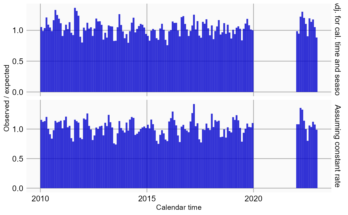

Ages covered per subject

We can visualize which age ranges are covered by each subject’s observation time:

plotAgeSpans(studyPop)

## Warning in plotAgeSpans(studyPop): There are 88453 cases. Random sampling 10000
## cases.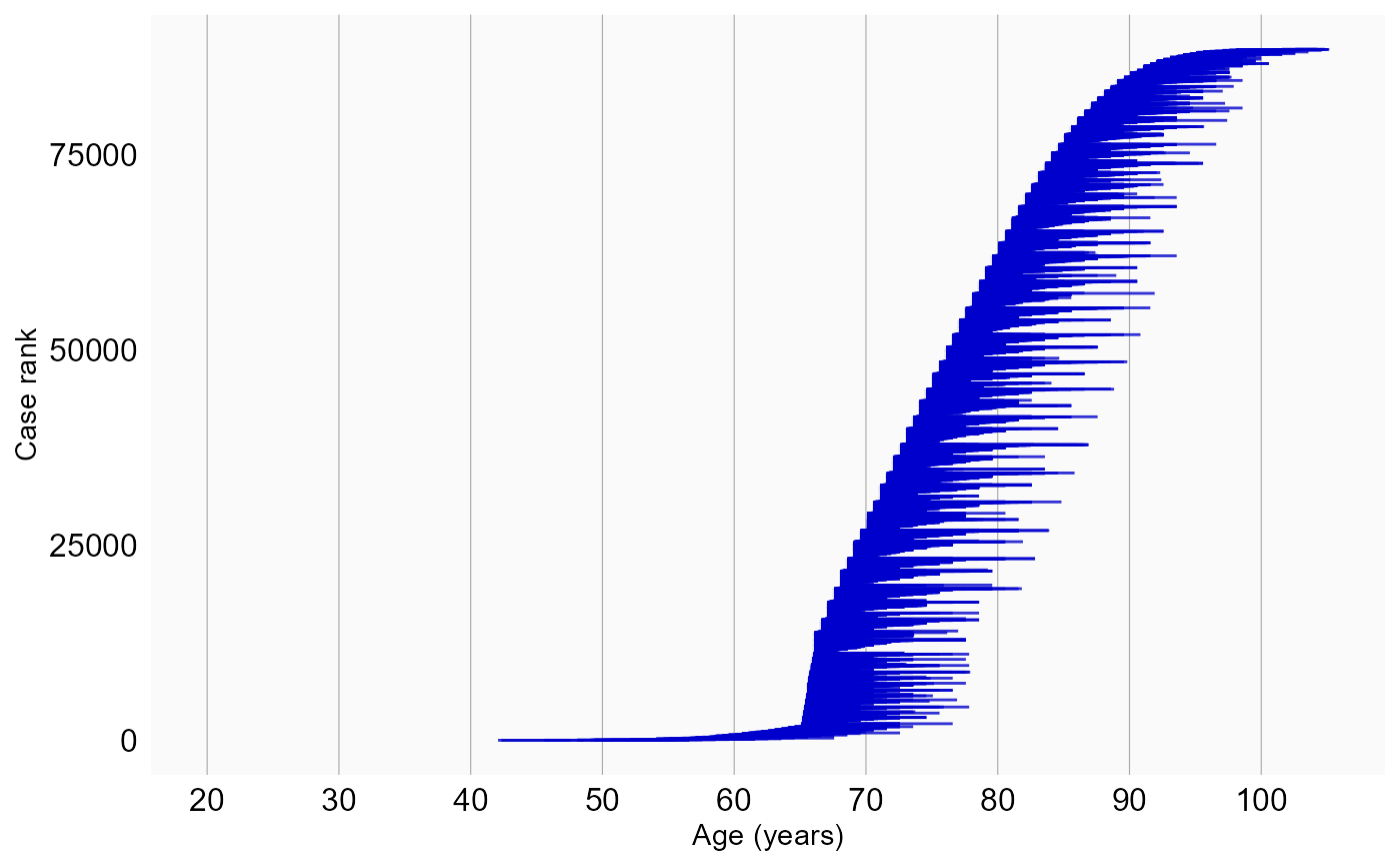

Here we see that most observation periods span only a small age range, making it unlikely that any within-person age-related effect will be large.

Acknowledgments

Considerable work has been dedicated to provide the SelfControlledCaseSeries package.

citation("SelfControlledCaseSeries")

## To cite package 'SelfControlledCaseSeries' in publications use:
## 
##   Schuemie M, Ryan P, Shaddox T, Suchard M (2025).
##   _SelfControlledCaseSeries: Self-Controlled Case Series_. R package
##   version 6.0.0, https://github.com/OHDSI/SelfControlledCaseSeries,
##   <https://ohdsi.github.io/SelfControlledCaseSeries/>.
## 
## A BibTeX entry for LaTeX users is
## 
##   @Manual{,
##     title = {SelfControlledCaseSeries: Self-Controlled Case Series},
##     author = {Martijn Schuemie and Patrick Ryan and Trevor Shaddox and Marc Suchard},
##     year = {2025},
##     note = {R package version 6.0.0, 
## https://github.com/OHDSI/SelfControlledCaseSeries},
##     url = {https://ohdsi.github.io/SelfControlledCaseSeries/},
##   }

Furthermore, SelfControlledCaseSeries makes extensive use of the Cyclops package.

citation("Cyclops")

## To cite Cyclops in publications use:
## 
##   Suchard MA, Simpson SE, Zorych I, Ryan P, Madigan D (2013). "Massive
##   parallelization of serial inference algorithms for complex
##   generalized linear models." _ACM Transactions on Modeling and
##   Computer Simulation_, *23*, 10. doi:10.1145/2414416.2414791
##   <https://doi.org/10.1145/2414416.2414791>.
## 
## A BibTeX entry for LaTeX users is
## 
##   @Article{,
##     author = {M. A. Suchard and S. E. Simpson and I. Zorych and P. Ryan and D. Madigan},
##     title = {Massive parallelization of serial inference algorithms for complex generalized linear models},
##     journal = {ACM Transactions on Modeling and Computer Simulation},
##     volume = {23},
##     pages = {10},
##     year = {2013},
##     doi = {10.1145/2414416.2414791},
##   }

Part of the code (related to event-dependent observation periods) is based on the SCCS package by Yonas Ghebremichael-Weldeselassie, Heather Whitaker, and Paddy Farrington.

This work is supported in part through the National Science Foundation grant IIS 1251151.

Martijn J. Schuemie, Marc A. Suchard and Patrick Ryan

2025-06-10