Plot empirical null distributions

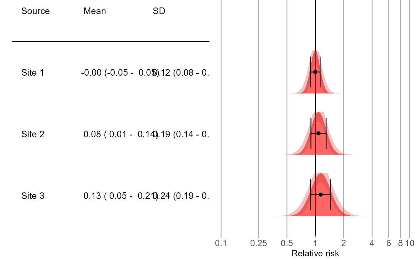
Plot the empirical null distribution for multiple data sources.

plotEmpiricalNulls(
  logRr,
  seLogRr,
  labels,
  xLabel = "Relative risk",
  limits = c(0.1, 10),
  showCis = TRUE,
  fileName = NULL
)

Arguments

logRr

A numeric vector of effect estimates for the negative controls on the log scale.

seLogRr

The standard error of the log of the effect estimates. Hint: often the standard error = (log(lower bound 95 percent confidence interval) - l og(effect estimate))/qnorm(0.025).

labels

A vector containing the labels for the various sources. Should be of equal length as logRr and seLogRr.

xLabel

The label on the x-axis: the name of the effect estimate.

limits

The limits of the effect size axis.

showCis

Show the 95 percent confidence intervals on the null distribution and distribution parameter estimates?

fileName

Name of the file where the plot should be saved, for example 'plot.png'. See the function ggplot2::ggsave() for supported file formats.

Value

A Ggplot object. Use the ggplot2::ggsave() function to save to file.

Details

Creates a plot showing the empirical null distributions. Distributions are shown as mean plus minus one standard deviation, as well as a distribution plot.

See also

EmpiricalCalibration::fitNull, EmpiricalCalibration::fitMcmcNull

Examples

# Some example data:
site1 <- EmpiricalCalibration::simulateControls(n = 50, mean = 0, sd = 0.1, trueLogRr = 0)
site1$label <- "Site 1"
site2 <- EmpiricalCalibration::simulateControls(n = 50, mean = 0.1, sd = 0.2, trueLogRr = 0)
site2$label <- "Site 2"
site3 <- EmpiricalCalibration::simulateControls(n = 50, mean = 0.15, sd = 0.25, trueLogRr = 0)
site3$label <- "Site 3"
sites <- rbind(site1, site2, site3)

plotEmpiricalNulls(logRr = sites$logRr, seLogRr = sites$seLogRr, labels = sites$label)