Code used in the video vignette

A short demonstration of the EvidenceSynthesis package

Martijn Schuemie

2025-10-15

This vignette contains the code used in a short video on the EvidenceSynthesis package: https://youtu.be/dho7E97vpgQ.

Simulate data

Simulate 10 sites:

simulationSettings <- createSimulationSettings(
  nSites = 10,
  n = 10000,
  treatedFraction = 0.8,
  nStrata = 5,
  hazardRatio = 2,
  randomEffectSd = 0.5
)
set.seed(1)
populations <- simulatePopulations(simulationSettings)

head(populations[[1]])

##   rowId stratumId x time y
## 1     1         5 1   10 0
## 2     2         2 1  113 0
## 3     3         4 1  135 0
## 4     4         2 1   27 0
## 5     5         2 1  104 0
## 6     6         3 1  342 0

table(populations[[1]][, c("x", "y")])

##    y
## x      0    1
##   0 1998    2
##   1 7981   19

Fit a model locally

Assume we are at site 1:

library(Cyclops)

population <- populations[[1]]

cyclopsData <- createCyclopsData(Surv(time, y) ~ x + strata(stratumId),
  data = population,
  modelType = "cox"
)
cyclopsFit <- fitCyclopsModel(cyclopsData)

# Hazard ratio:
exp(coef(cyclopsFit))

##        x 
## 2.378318

# 95% confidence interval:
exp(confint(cyclopsFit, parm = "x")[2:3])

## [1]  0.6888127 14.9382268

Approximate the likelihood function at one site

Normal approximation

normalApproximation <- approximateLikelihood(
  cyclopsFit = cyclopsFit,
  parameter = "x",
  approximation = "normal"
)
normalApproximation

##         rr    ci95Lb   ci95Ub     logRr   seLogRr
## x 2.378318 0.6888127 14.93823 0.8663934 0.7848893

plotLikelihoodFit(
  approximation = normalApproximation,
  cyclopsFit = cyclopsFit,
  parameter = "x"
)

## Detected data following normal distribution

## Warning: Using `size` aesthetic for lines was deprecated in ggplot2 3.4.0.
## ℹ Please use `linewidth` instead.
## ℹ The deprecated feature was likely used in the EvidenceSynthesis package.
##   Please report the issue at
##   <https://github.com/OHDSI/EvidenceSynthesis/issues>.
## This warning is displayed once every 8 hours.
## Call `lifecycle::last_lifecycle_warnings()` to see where this warning was
## generated.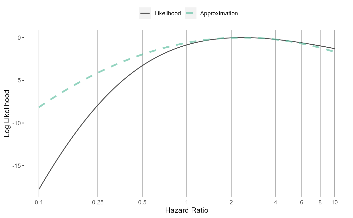

Adaptive approximation

approximation <- approximateLikelihood(
  cyclopsFit = cyclopsFit,
  parameter = "x",
  approximation = "adaptive grid",
  bounds = c(log(0.1), log(10))
)
head(approximation)

## # A tibble: 6 × 2
##   point value
##   <dbl> <dbl>
## 1 -2.30 -156.
## 2 -2.29 -156.
## 3 -2.27 -156.
## 4 -2.25 -155.
## 5 -2.24 -155.
## 6 -2.22 -155.

plotLikelihoodFit(
  approximation = approximation,
  cyclopsFit = cyclopsFit,
  parameter = "x"
)

## Detected data following adaptive grid distribution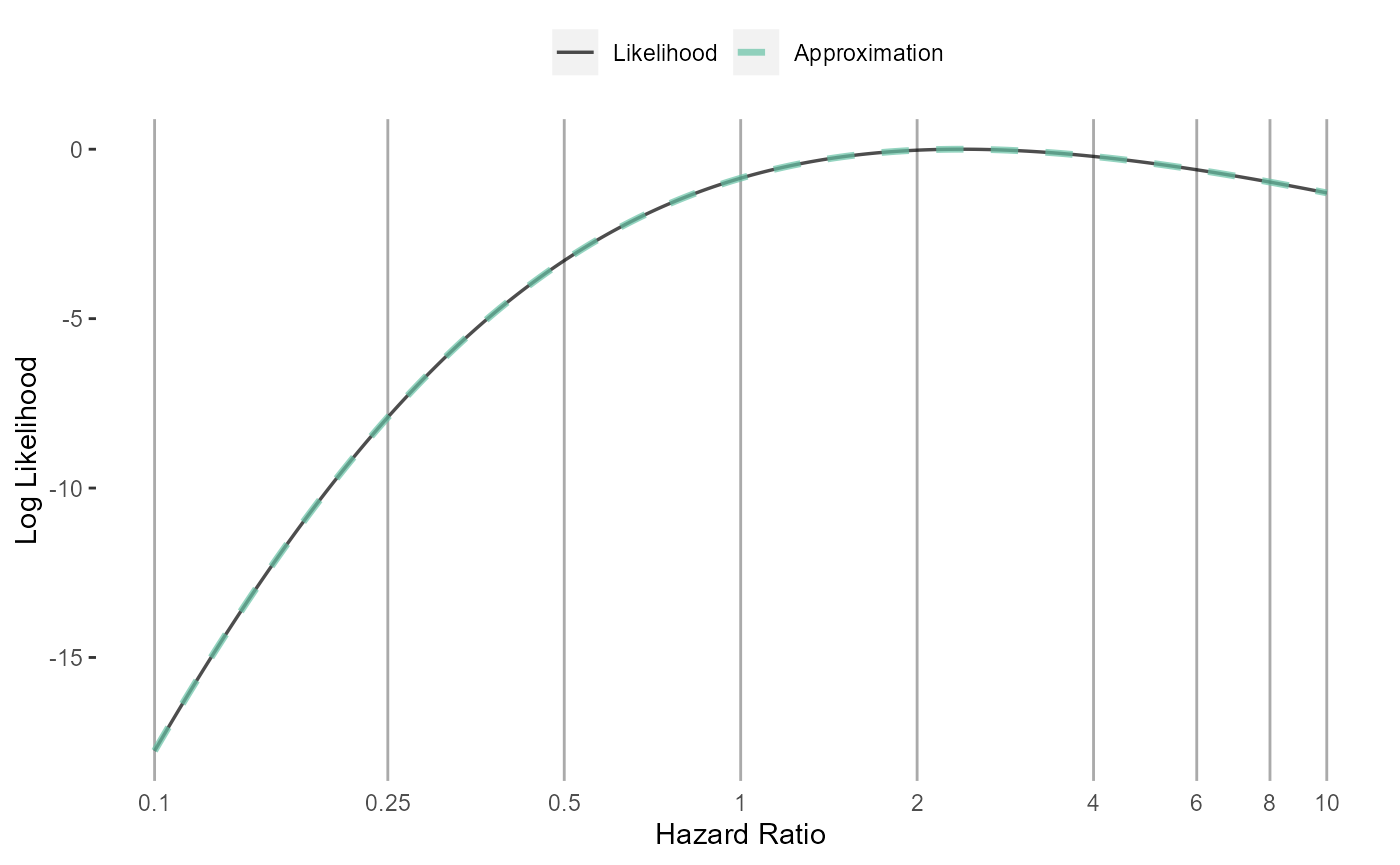

Approximate at all sites

fitModelInDatabase <- function(population, approximation) {
  cyclopsData <- createCyclopsData(Surv(time, y) ~ x + strata(stratumId),
    data = population,
    modelType = "cox"
  )
  cyclopsFit <- fitCyclopsModel(cyclopsData)
  approximation <- approximateLikelihood(cyclopsFit,
    parameter = "x",
    approximation = approximation
  )
  return(approximation)
}
adaptiveGridApproximations <- lapply(
  X = populations,
  FUN = fitModelInDatabase,
  approximation = "adaptive grid"
)
normalApproximations <- lapply(
  X = populations,
  FUN = fitModelInDatabase,
  approximation = "normal"
)
normalApproximations <- do.call(rbind, (normalApproximations))

Synthesize evidence

Fixed-effects

Gold standard (pooling data):

fixedFxPooled <- computeFixedEffectMetaAnalysis(populations)
fixedFxPooled

##         rr       lb       ub     logRr  seLogRr
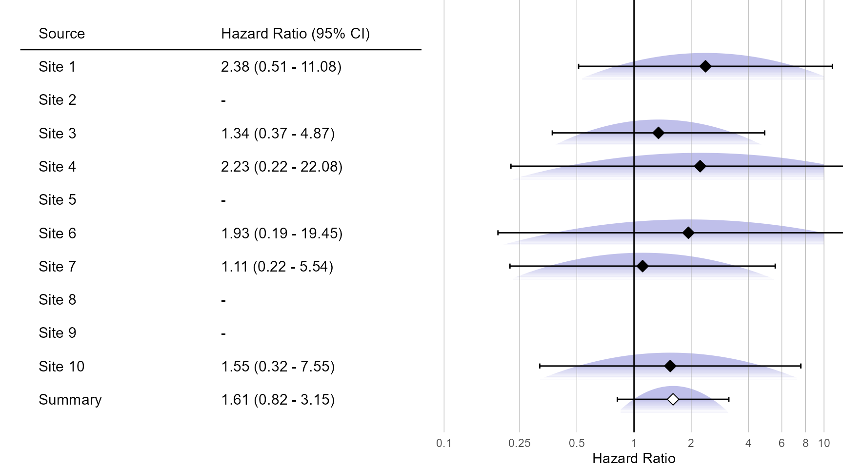
## x 2.432933 1.370034 4.800644 0.8890975 0.319882

Normal approximation:

fixedFxNormal <- computeFixedEffectMetaAnalysis(normalApproximations)

## Warning: Estimate(s) with NA seLogRr detected. Removing before computing
## meta-analysis.

## Warning: Estimate(s) with extremely high seLogRr (>100) detected. Removing
## before computing meta-analysis.

fixedFxNormal

##         rr        lb       ub     logRr   seLogRr
## 1 1.605267 0.8168054 3.154828 0.4732898 0.3447228

Adaptive grid approximation:

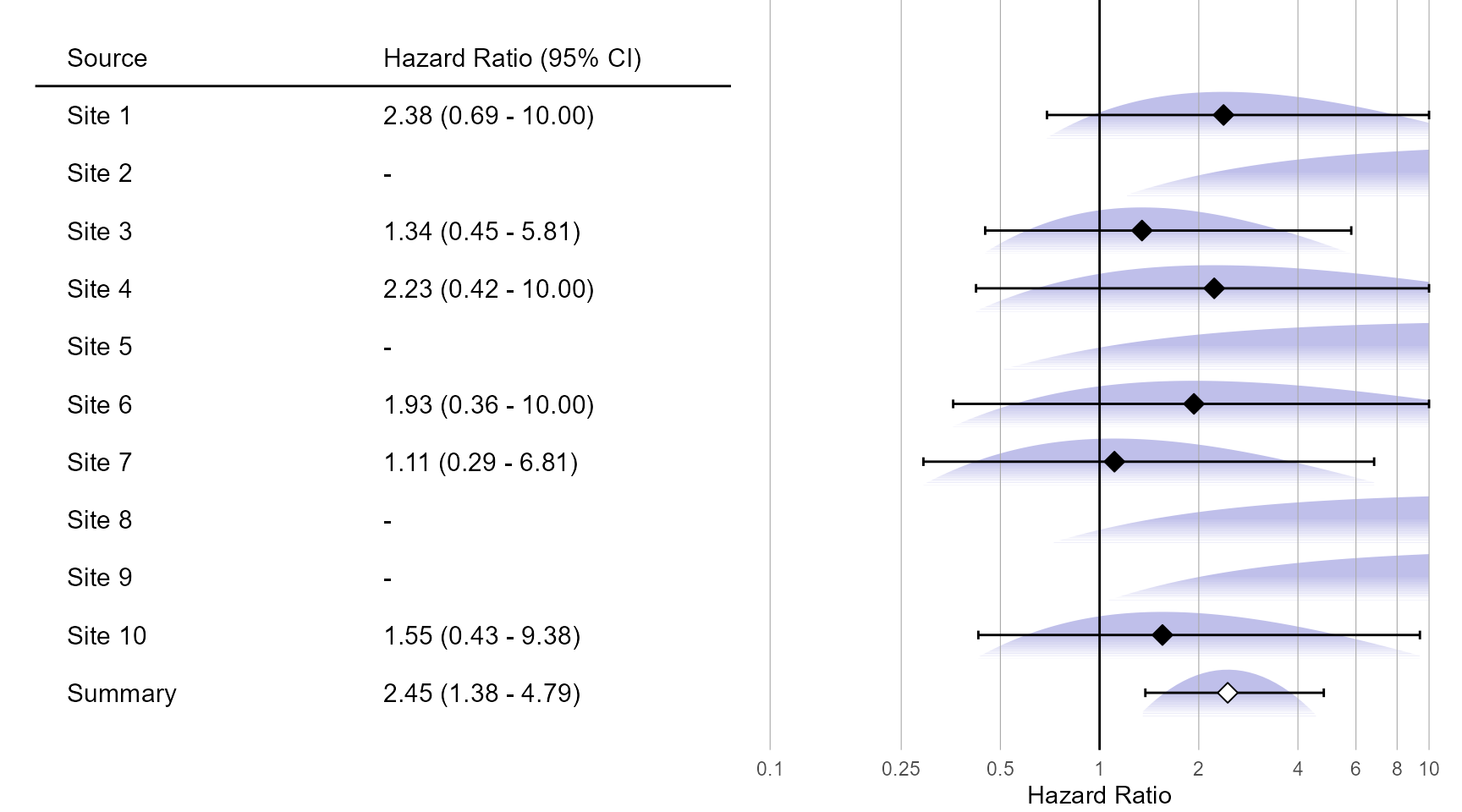
fixedFxAdaptiveGrid <- computeFixedEffectMetaAnalysis(adaptiveGridApproximations)
fixedFxAdaptiveGrid

##         rr       lb       ub     logRr   seLogRr
## 1 2.448437 1.376857 4.792428 0.8954498 0.3181777

Visualization

Normal approximation:

plotMetaAnalysisForest(
  data = normalApproximations,
  labels = paste("Site", 1:10),
  estimate = fixedFxNormal,
  xLabel = "Hazard Ratio"
)

Adaptive grid approximation:

plotMetaAnalysisForest(
  data = adaptiveGridApproximations,
  labels = paste("Site", 1:10),
  estimate = fixedFxAdaptiveGrid,
  xLabel = "Hazard Ratio"
)

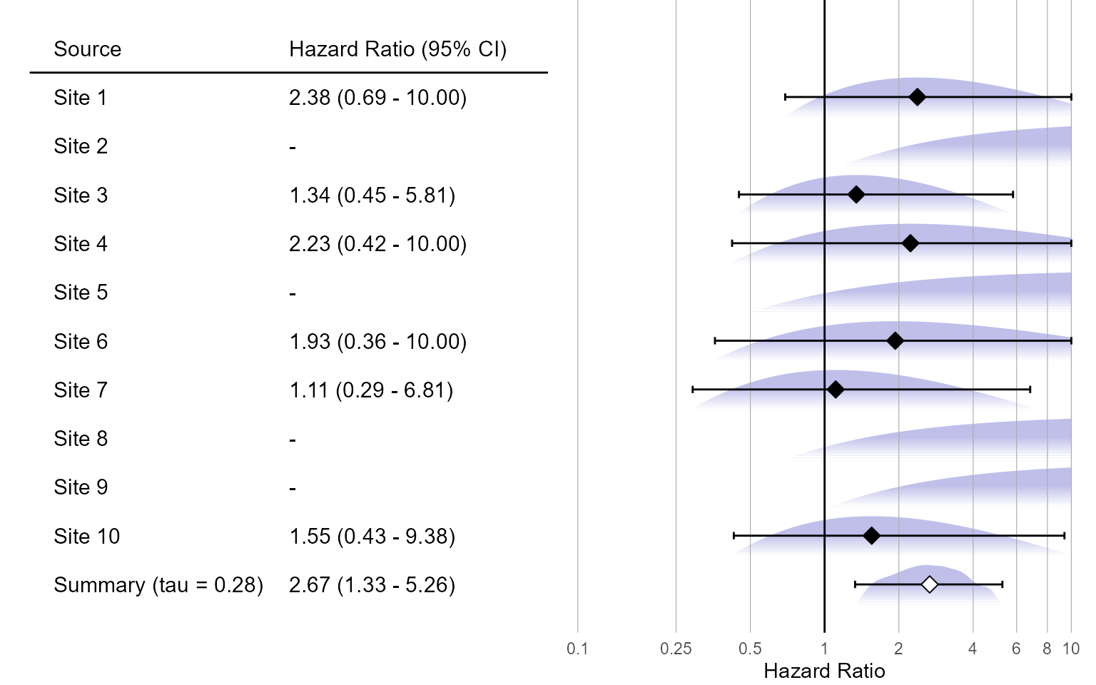
Random-effects

Gold standard (pooling data):

randomFxPooled <- computeBayesianMetaAnalysis(populations)
exp(randomFxPooled[, 1:3])

##         mu   mu95Lb   mu95Ub
## 1 2.705529 1.416858 5.465772

Normal approximation:

randomFxNormal <- computeBayesianMetaAnalysis(normalApproximations)

## Warning: Estimate(s) with NA seLogRr detected. Removing before computing
## meta-analysis.

## Warning: Estimate(s) with extremely high seLogRr (>100) detected. Removing
## before computing meta-analysis.

exp(randomFxNormal[, 1:3])

##         mu    mu95Lb   mu95Ub
## 1 1.597623 0.7221914 3.083936

Adaptive grid approximation:

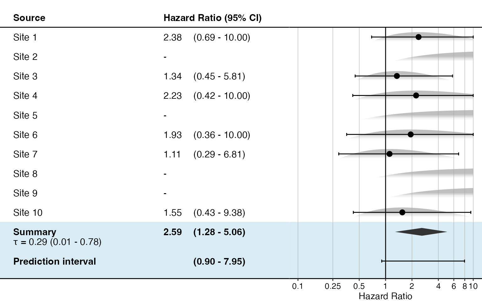
randomFxAdaptiveGrid <- computeBayesianMetaAnalysis(adaptiveGridApproximations)
exp(randomFxAdaptiveGrid[, 1:3])

##        mu   mu95Lb   mu95Ub
## 1 2.59455 1.283359 5.064328

Visualization

Normal approximation:

plotMetaAnalysisForest(
  data = normalApproximations,
  labels = paste("Site", 1:10),
  estimate = randomFxNormal,
  xLabel = "Hazard Ratio"
)

Adaptive grid approximation:

plotMetaAnalysisForest(
  data = adaptiveGridApproximations,
  labels = paste("Site", 1:10),
  estimate = randomFxAdaptiveGrid,
  xLabel = "Hazard Ratio"
)