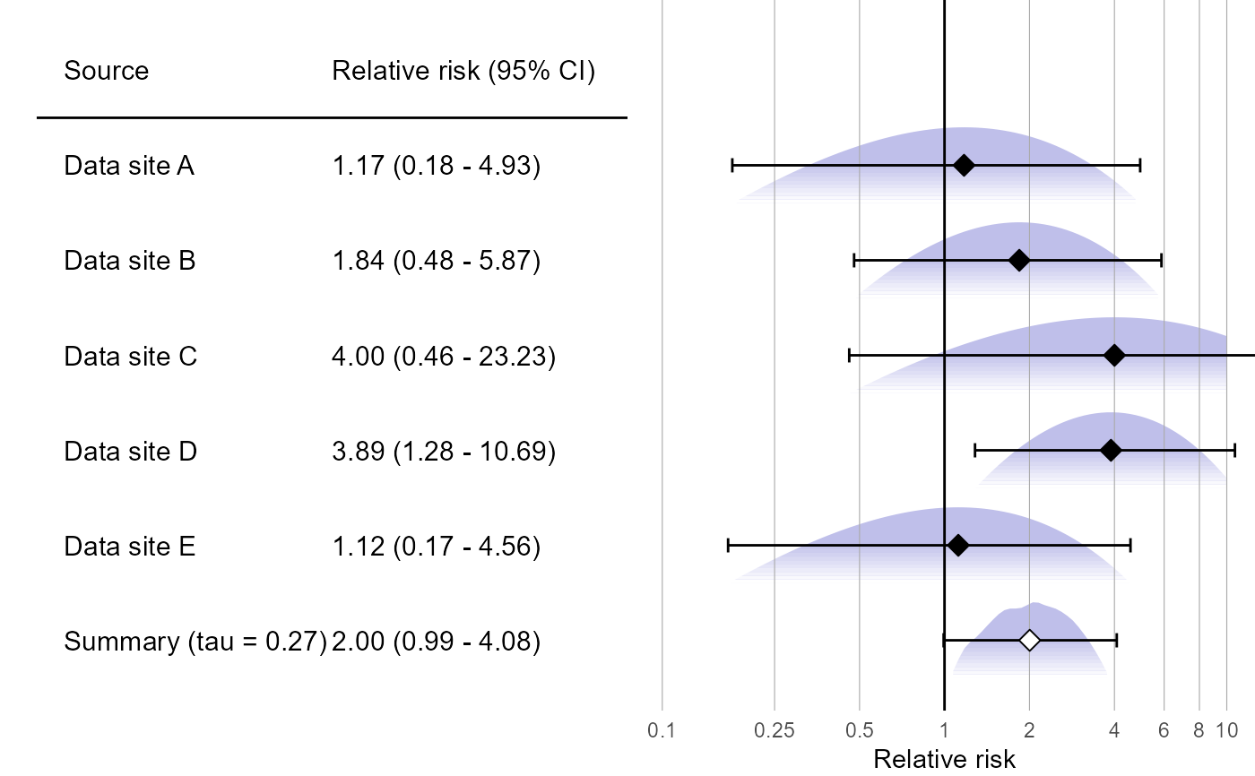
Creates a forest plot of effect size estimates, including the summary estimate.
plotMetaAnalysisForest(
  data,
  labels,
  estimate,
  xLabel = "Relative risk",
  summaryLabel = "Summary",
  limits = c(0.1, 10),
  alpha = 0.05,
  showPredictionInterval = TRUE,
  showLikelihood = TRUE,
  fileName = NULL
)
Arguments
- data
A data frame containing either normal, skew-normal, custom parametric, or grid likelihood data. One row per database.
- labels
A vector of labels for the data sources.
- estimate
The meta-analytic estimate as created using either computeFixedEffectMetaAnalysis or computeBayesianMetaAnalysis function.
- xLabel
The label on the x-axis: the name of the effect estimate.
- summaryLabel
The label for the meta-analytic estimate.
- limits
The limits of the effect size axis.
- alpha
The alpha (expected type I error).
- showPredictionInterval
Show the prediction interval (for random effects models).
- showLikelihood
Show the likelihood curve for each estimate?
- fileName
Name of the file where the plot should be saved, for example 'plot.png'. See the function ggplot2::ggsave ifor supported file formats.
Value
A Ggplot object. Use the ggplot2::ggsave function to save to file.
Details
Creates a forest plot of effect size estimates, including a meta-analysis estimate.
Examples
# Simulate some data for this example:
populations <- simulatePopulations()
labels <- paste("Data site", LETTERS[1:length(populations)])

# Fit a Cox regression at each data site, and approximate likelihood function:
fitModelInDatabase <- function(population) {
  cyclopsData <- Cyclops::createCyclopsData(Surv(time, y) ~ x + strata(stratumId),
    data = population,
    modelType = "cox"
  )
  cyclopsFit <- Cyclops::fitCyclopsModel(cyclopsData)
  approximation <- approximateLikelihood(cyclopsFit,
                                         parameter = "x",
                                         approximation = "grid with gradients")
  return(approximation)
}
approximations <- lapply(populations, fitModelInDatabase)

# At study coordinating center, perform meta-analysis using per-site approximations:
estimate <- computeBayesianMetaAnalysis(approximations)
#> Detected data following grid with gradients distribution
#> Performing MCMC. This may take a while
plotMetaAnalysisForest(approximations, labels, estimate)


# (Estimates in this example will vary due to the random simulation)