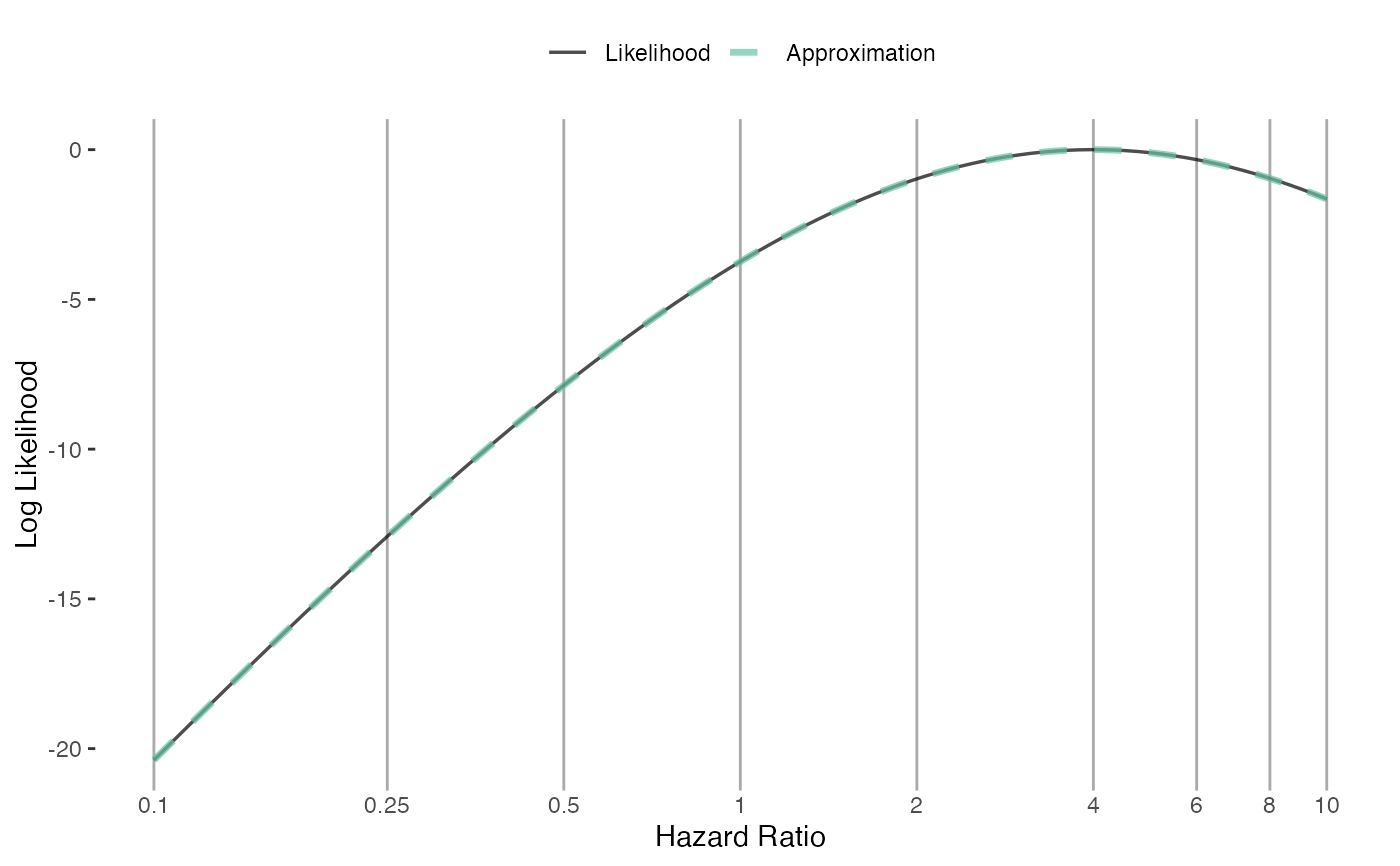
Plot the likelihood approximation

plotLikelihoodFit(
  approximation,
  cyclopsFit,
  parameter = "x",
  logScale = TRUE,
  xLabel = "Hazard Ratio",
  limits = c(0.1, 10),
  fileName = NULL
)

Arguments

approximation: An approximation of the likelihood function as fitted using the approximateLikelihood() function.
cyclopsFit: A model fitted using the Cyclops::fitCyclopsModel() function.
parameter: The parameter in the cyclopsFit object to profile.
logScale: Show the y-axis on the log scale?
xLabel: The title of the x-axis.
limits: The limits on the x-axis.
fileName: Name of the file where the plot should be saved, for example 'plot.png'. See the function ggplot2::ggsave in the ggplot2 package for supported file formats.

Value

A Ggplot object. Use the ggplot2::ggsave function to save to file.

Details

Plots the (log) likelihood and the approximation of the likelihood. Allows for reviewing the approximation.

Examples

# Simulate a single database population:
population <- simulatePopulations(createSimulationSettings(nSites = 1))[[1]]

# Approximate the likelihood:
cyclopsData <- Cyclops::createCyclopsData(Surv(time, y) ~ x + strata(stratumId),
  data = population,
  modelType = "cox"
)
cyclopsFit <- Cyclops::fitCyclopsModel(cyclopsData)
approximation <- approximateLikelihood(cyclopsFit, parameter = "x", approximation = "custom")

plotLikelihoodFit(approximation, cyclopsFit, parameter = "x")
#> Detected data following custom parameric distribution