Summarising measurement use in a dataset
Source:vignettes/a01_summariseMeasurementUse.Rmd
a01_summariseMeasurementUse.RmdIntroduction
In this vignette we will see how we can summarise the use of measurement concepts in our dataset as a whole. For our example we’re going to be interested in measurement concepts related to respiratory function and will use the Eunomia synthetic dataset.
First we will connect to the database and create a cdm reference.
con <- dbConnect(duckdb(), dbdir = eunomiaDir())
#> Creating CDM database /tmp/RtmpZhVMWq/GiBleed_5.3.zip
cdm <- cdmFromCon(
  con = con, cdmSchem = "main", writeSchema = "main", cdmName = "Eunomia"
)
cdm
#>
#> ── # OMOP CDM reference (duckdb) of Eunomia ────────────────────────────────────
#> • omop tables: care_site, cdm_source, concept, concept_ancestor, concept_class,
#> concept_relationship, concept_synonym, condition_era, condition_occurrence,
#> cost, death, device_exposure, domain, dose_era, drug_era, drug_exposure,
#> drug_strength, fact_relationship, location, measurement, metadata, note,
#> note_nlp, observation, observation_period, payer_plan_period, person,
#> procedure_occurrence, provider, relationship, source_to_concept_map, specimen,
#> visit_detail, visit_occurrence, vocabulary
#> • cohort tables: -
#> • achilles tables: -
#> • other tables: -
Defining a codelist of measurements
Now we’ll create a codelist with measurement concepts.
respiratory_function_codes <- newCodelist(list(
  "respiratory_function" = c(4052083L, 4133840L, 3011505L)
))
respiratory_function_codes
#>
#> - respiratory_function (3 codes)
For a general summary of the use of these codes in our dataset we can
use summariseCodeUse from the CodelistGenerator
R package.
library(CodelistGenerator)
code_use <- summariseCodeUse(respiratory_function_codes, cdm)
tableCodeUse(code_use)|
Database name
|
|||||||||||
|---|---|---|---|---|---|---|---|---|---|---|---|
|
Eunomia
|
|||||||||||
| Codelist name | Standard concept name | Standard concept ID | Source concept name | Source concept ID | Source concept value | Type concept id | Type concept name | Domain ID | Table |
Estimate name
|
|
| Record count | Person count | ||||||||||
| respiratory_function | overall | – | NA | NA | NA | NA | NA | NA | NA | 8,728 | 2,096 |
| Measurement of respiratory function | 4052083 | Measurement of respiratory function | 4052083 | 23426006 | 5001 | NA | measurement | measurement | 4,088 | 2,072 | |
| FEV1/FVC | 3011505 | FEV1/FVC | 3011505 | 19926-5 | 5001 | NA | measurement | measurement | 2,320 | 125 | |
| Spirometry | 4133840 | Spirometry | 4133840 | 127783003 | 5001 | NA | measurement | measurement | 2,320 | 125 | |
While this provides a useful high-level summary, more detailed information is often needed to assess study feasibility and design.
Measurement diagnostics
The MeasurementDiagnostics package provides additional, measurement-specific diagnostic checks. Specifically, it includes three types of diagnostics:
measurement_summary: summarises the number of subjects with measurements, the number of measurements per subject, and the time between measurements.measurement_value_as_number: summarises measurement values recorded as numeric values, providing descriptive statistics by measurement unit.measurement_value_as_concept: summarises measurement values recorded as concepts and their frequencies.
These diagnostics can be performed using the
summariseMeasurementUse() function.
library(MeasurementDiagnostics)

respiratory_function_measurements <- summariseMeasurementUse(
  cdm = cdm,
  codes = respiratory_function_codes
)
As with some other OMOP analytical packages, results are returned in
the summarised_result format defined by the omopgenerics
package.
respiratory_function_measurements |>
  glimpse()
#> Rows: 2,116
#> Columns: 13
#> $ result_id        <int> 1, 1, 1, 1, 1, 1, 1, 1, 1, 1, 1, 1, 1, 1, 1, 1, 1, 1,…
#> $ cdm_name         <chr> "Eunomia", "Eunomia", "Eunomia", "Eunomia", "Eunomia"…
#> $ group_name       <chr> "codelist_name", "codelist_name", "codelist_name", "c…
#> $ group_level      <chr> "respiratory_function", "respiratory_function", "resp…
#> $ strata_name      <chr> "overall", "overall", "overall", "overall", "overall"…
#> $ strata_level     <chr> "overall", "overall", "overall", "overall", "overall"…
#> $ variable_name    <chr> "number_subjects", "days_between_measurements", "days…
#> $ variable_level   <chr> NA, NA, NA, NA, NA, NA, "density_001", "density_001",…
#> $ estimate_name    <chr> "count", "min", "q25", "median", "q75", "max", "densi…
#> $ estimate_type    <chr> "integer", "integer", "integer", "integer", "integer"…
#> $ estimate_value   <chr> "2096", "0", "0", "371", "1726", "33541", "0", "0.000…
#> $ additional_name  <chr> "overall", "overall", "overall", "overall", "overall"…
#> $ additional_level <chr> "overall", "overall", "overall", "overall", "overall"…
Visualise results
For each diagnostic check, the package provides both
table and plot functions. For example,
the following table displays results from the
measurement_summary check:
tableMeasurementSummary(respiratory_function_measurements)| CDM name | Codelist name | Variable name | Estimate name | Estimate value |
|---|---|---|---|---|
| Eunomia | respiratory_function | Number subjects | N (%) | 2,096 (77.80%) |
| Days between measurements | Median [Q25 – Q75] | 371 [0 – 1,726] | ||
| Range | 0 to 33,541 | |||
| Measurements per subject | Median [Q25 – Q75] | 2.00 [1.00 – 3.00] | ||
| Range | 1.00 to 138.00 |
To learn more about available tables and plots, see the vignette “Results Visualisation”.
Stratifications
By default, summariseMeasurementUse() stratifies results
by codelist only. That is, all checks are returned for the overall
codelist, and the value-based checks
(measurement_value_as_number and
measurement_value_as_concept) are further stratified by
individual measurement concepts.
However, results can also be stratified by sex, year of measurement,
and age group at measurement date In the following example, we generate
measurement_value_as_number results stratified by sex and
two different age group definitions.
results <- summariseMeasurementUse(
  cdm = cdm,
  codes = respiratory_function_codes,
  byConcept = FALSE,
  byYear = FALSE,
  bySex = TRUE,
  ageGroup = list(
    age_group_narrow = list(c(0, 19), c(20, 39), c(40, 59), c(60, 79), c(80, 150)),
    age_group_broad = list(c(0, 17), c(18, 64), c(65, 150))
  ),
  checks = "measurement_value_as_number"
)

# Show results stratified by broad age group
results |>
  filterStrata(age_group_broad != "overall") |>
  tableMeasurementValueAsNumber(
    header = "age_group_broad",
    groupColumn = character(),
    hide = c("age_group_narrow", "sex", "variable_level")
)| CDM name | Codelist name | Unit concept name | Unit concept ID | Variable name | Estimate name |
Age group broad
|
||
|---|---|---|---|---|---|---|---|---|
| 0 to 17 | 18 to 64 | 65 to 150 | ||||||
| Eunomia | respiratory_function | No matching concept | 0 | Measurement records | N | 1,396 | 5,787 | 1,545 |
| Value as number | Median [Q25 – Q75] | – | – | – | ||||
| Q05 – Q95 | – | – | – | |||||
| Q01 – Q99 | – | – | – | |||||
| Range | – | – | – | |||||
| Missing value, N (%) | 1,396 (100.00%) | 5,787 (100.00%) | 1,545 (100.00%) | |||||
Estimates
By default, each diagnostic check produces a predefined set of estimates. These can be modified using the estimates argument.
The default estimates are:
1. measurement_summary: "min",
"q25", "median", "q75",
"max", "density"
2. measurement_value_as_number: "min",
"q01", "q05", "q25",
"median", "q75", "q95",
"q99", "max", "count_missing",
"percentage_missing", "density"
3. measurement_value_as_concept:
"count", "percentage"
Allowed estimates depend on the type of variable being summarised.
For example, measurement_value_as_concept only supports
categorical estimates, whereas the others use numeric estimates (as
variables are numeric, e.g. time between measurements).
Available estimates are defined in the PatientProfiles
package. To see all supported estimates and their naming conventions,
use availableEstimates() from that package. Note that only
categorical estimates are allowed for
measurement_value_as_concept, while the other checks only
allow estimates for numeric variable types.
In the following example, we run all checks without density estimates and with a reduced set of quantiles:
results <- summariseMeasurementUse(
  cdm = cdm,
  codes = respiratory_function_codes,
  estimates = list(
    measurement_summary = c("min", "q25", "median", "q75", "max"),
    measurement_value_as_number = c(
      "min", "q25", "median", "q75", "max",
      "count_missing", "percentage_missing"
    ),
    measurement_value_as_concept = c("count", "percentage")
  )
)

results |>
tableMeasurementValueAsNumber()| CDM name | Concept name | Concept ID | Source concept name | Source concept ID | Domain ID | Unit concept name | Unit concept ID | Variable name | Estimate name | Estimate value |
|---|---|---|---|---|---|---|---|---|---|---|
| respiratory_function | ||||||||||
| Eunomia | overall | overall | overall | overall | overall | No matching concept | 0 | Measurement records | N | 8,728 |
| Value as number | Median [Q25 – Q75] | – | ||||||||
| Range | – | |||||||||
| Missing value, N (%) | 8,728 (100.00%) | |||||||||
| Measurement of respiratory function | 4052083 | Measurement of respiratory function | 4052083 | Measurement | No matching concept | 0 | Measurement records | N | 4,088 | |
| Value as number | Median [Q25 – Q75] | – | ||||||||
| Range | – | |||||||||
| Missing value, N (%) | 4,088 (100.00%) | |||||||||
| FEV1/FVC | 3011505 | FEV1/FVC | 3011505 | Measurement | No matching concept | 0 | Measurement records | N | 2,320 | |
| Value as number | Median [Q25 – Q75] | – | ||||||||
| Range | – | |||||||||
| Missing value, N (%) | 2,320 (100.00%) | |||||||||
| Spirometry | 4133840 | Spirometry | 4133840 | Measurement | No matching concept | 0 | Measurement records | N | 2,320 | |
| Value as number | Median [Q25 – Q75] | – | ||||||||
| Range | – | |||||||||
| Missing value, N (%) | 2,320 (100.00%) | |||||||||
Histogram estimates
Histogram-style summaries can be obtained using the
histogram argument. This allows users to specify custom
bins for the following variables:
"days_between_measurements""measurements_per_subject""value_as_number"
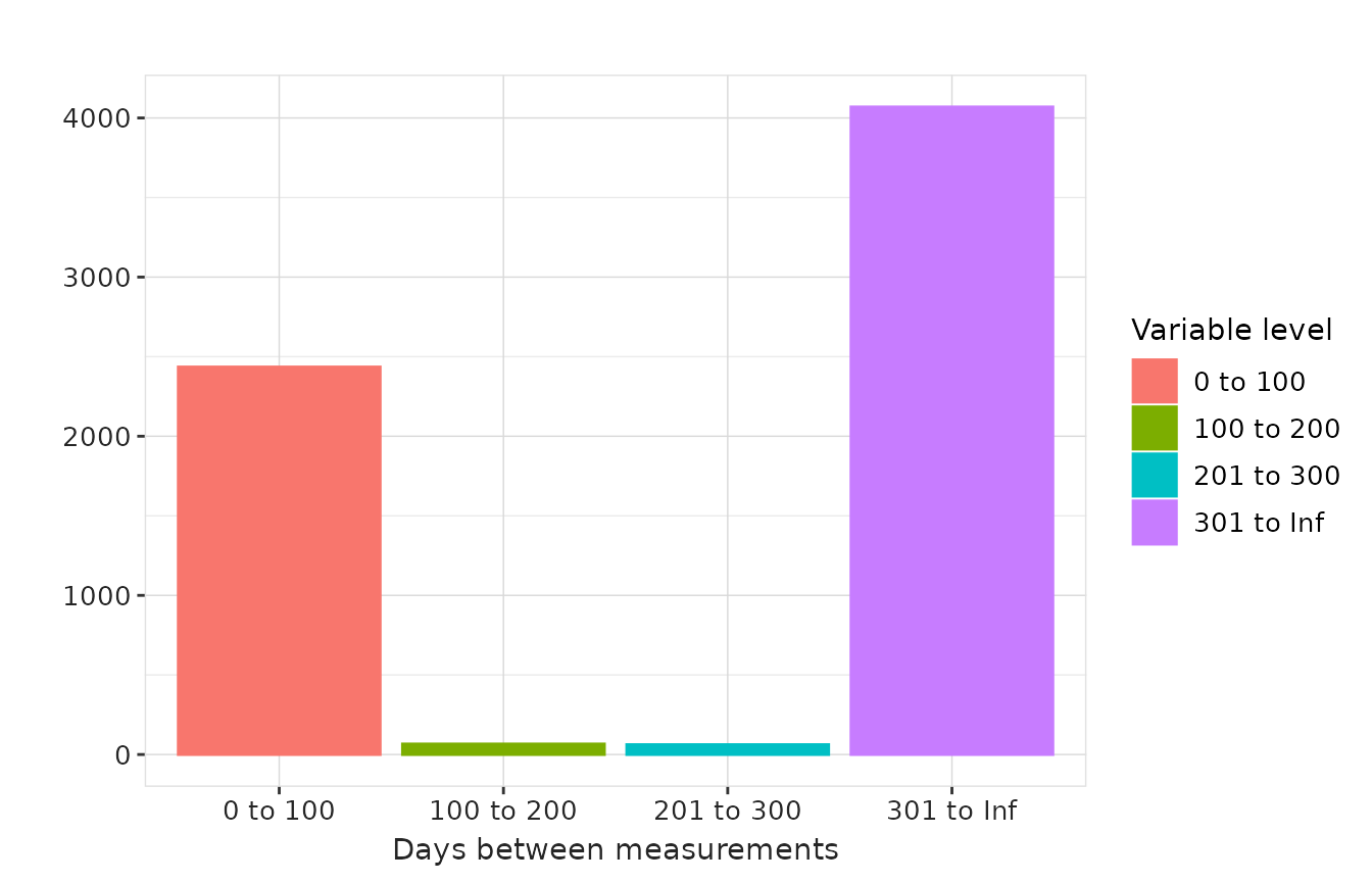
In the example below, we generate histogram summaries for days between measurements and measurements per subject using custom bandwidths.
results <- summariseMeasurementUse(
  cdm = cdm,
  codes = respiratory_function_codes,
  estimates = NULL,
  histogram = list(
    "days_between_measurements" = list(
      '0 to 100' = c(0, 100), '100 to 200' = c(101, 200),
      '201 to 300' = c(201, 300), '301 to Inf' = c(301, Inf)
    ),
    "measurements_per_subject" = list(
      '0 to 1' = c(0, 1), '2 to 3' = c(2, 3),
      '4 to 5' = c(4, 5), '6 to 7' = c(6, 7),
      '8+' = c(8, 1000)
    )
  )
)

results |>
  plotMeasurementSummary(
    x = "variable_level",
    plotType = "barplot",
    colour = "variable_level"
  )
results |>
  plotMeasurementSummary(
    x = "variable_level",
    y = "measurements_per_subject",
    plotType = "barplot",
    colour = "variable_level"
  )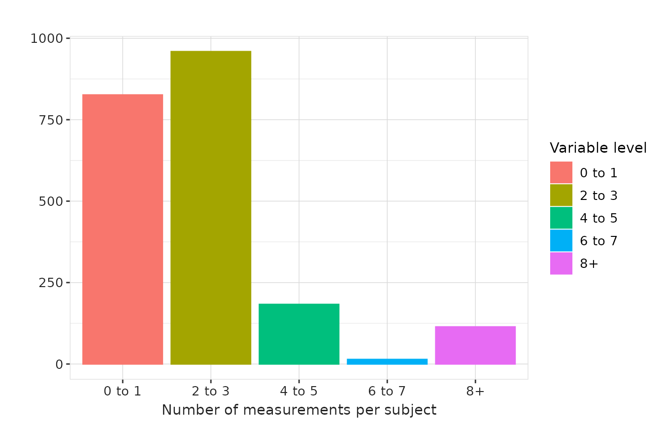
Note that density and histogram estimates do not appear in tables, these are just visualised in plot functions by using the plot types “densityplot” and “barplot” respectively.
Other arguments
The study period can be restricted using the dateRange
argument. In addition, to reduce computational time, diagnostics are by
default performed on a random sample of 20,000 persons. This sample size
can be modified using personSample, or sampling can be
disabled entirely by setting personSample = NULL.