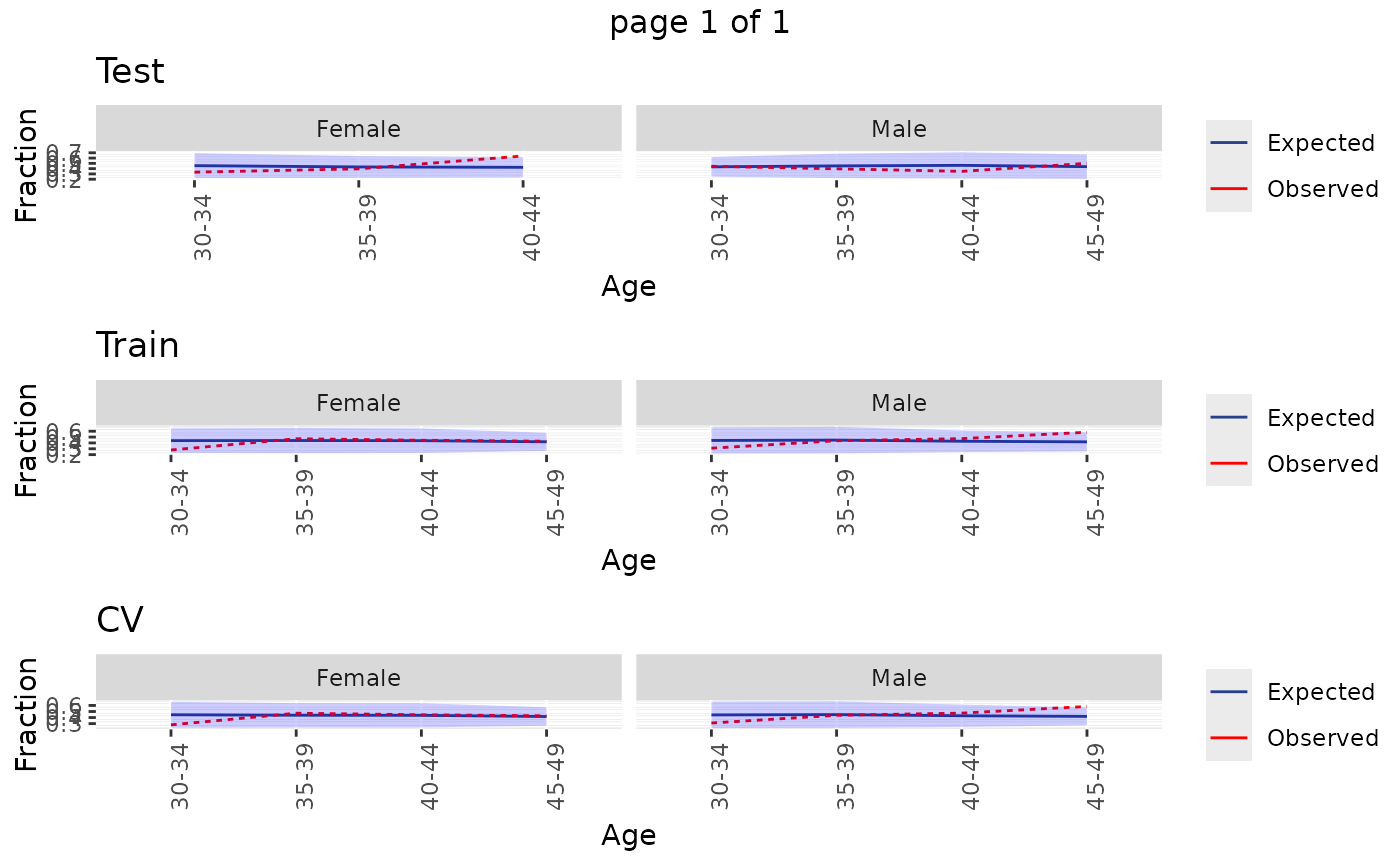
Plot the Observed vs. expected incidence, by age and gender

Usage

plotDemographicSummary(
  plpResult,
  typeColumn = "evaluation",
  saveLocation = NULL,
  fileName = "roc.png"
)

Arguments

plpResult: A plp result object as generated using the runPlp function.
typeColumn: The name of the column specifying the evaluation type
saveLocation: Directory to save plot (if NULL plot is not saved)
fileName: Name of the file to save to plot, for example 'plot.png'. See the function ggsave in the ggplot2 package for supported file formats.

Value

A ggplot object. Use the ggsave function to save to file in a different format.

Details

Create a plot showing the Observed vs. expected incidence, by age and gender #'

Examples

# \donttest{
data("simulationProfile")
plpData <- simulatePlpData(simulationProfile, n = 1000, seed = 42)
#> Generating covariates
#> Generating cohorts
#> Generating outcomes
saveLoc <- file.path(tempdir(), "plotDemographicSummary")
plpResult <- runPlp(plpData, outcomeId = 3, saveDirectory = saveLoc)
#> Use timeStamp: TRUE
#> Creating save directory at: /tmp/Rtmpb7S9Xv/plotDemographicSummary/2025-10-02-3
#> Currently in a tryCatch or withCallingHandlers block, so unable to add global calling handlers. ParallelLogger will not capture R messages, errors, and warnings, only explicit calls to ParallelLogger. (This message will not be shown again this R session)
#> Patient-Level Prediction Package version 6.5.0
#> Study started at: 2025-10-02 13:01:31.418994
#> AnalysisID:         2025-10-02-3
#> AnalysisName:       Study details
#> TargetID:           1
#> OutcomeID:          3
#> Cohort size:        1000
#> Covariates:         98
#> Creating population
#> Outcome is 0 or 1
#> Population created with: 954 observations, 954 unique subjects and 434 outcomes
#> Population created in 0.0571 secs
#> seed: 123
#> Creating a 25% test and 75% train (into 3 folds) random stratified split by class
#> Data split into 238 test cases and 716 train cases (239, 239, 238)
#> Data split in 0.574 secs
#> Train Set:
#> Fold 1 239 patients with 109 outcomes - Fold 2 239 patients with 109 outcomes - Fold 3 238 patients with 108 outcomes
#> 66 covariates in train data
#> Test Set:
#> 238 patients with 108 outcomes
#> Removing 2 redundant covariates
#> Removing 0 infrequent covariates
#> Normalizing covariates
#> Tidying covariates took 0.818 secs
#> Train Set:
#> Fold 1 239 patients with 109 outcomes - Fold 2 239 patients with 109 outcomes - Fold 3 238 patients with 108 outcomes
#> 64 covariates in train data
#> Test Set:
#> 238 patients with 108 outcomes
#> 
#> Running Cyclops
#> Done.
#> GLM fit status:  OK
#> Creating variable importance data frame
#> Prediction took 0.168 secs
#> Time to fit model: 0.391 secs
#> Removing infrequent and redundant covariates and normalizing
#> Removing infrequent and redundant covariates covariates and normalizing took 0.171 secs
#> Prediction took 0.175 secs
#> Prediction done in: 0.51 secs
#> Calculating Performance for Test
#> =============
#> AUC                 60.80
#> 95% lower AUC:      53.84
#> 95% upper AUC:      67.77
#> AUPRC:              56.81
#> Brier:              0.23
#> Eavg:               0.10
#> Calibration in large- Mean predicted risk 0.4487 : observed risk 0.4538
#> Calibration in large- Intercept 0.226
#> Weak calibration intercept: 0.226 - gradient:1.937
#> Hosmer-Lemeshow calibration gradient: 1.43 intercept:         -0.18
#> Average Precision:  0.58
#> Calculating Performance for Train
#> =============
#> AUC                 59.44
#> 95% lower AUC:      55.38
#> 95% upper AUC:      63.50
#> AUPRC:              55.19
#> Brier:              0.24
#> Eavg:               0.02
#> Calibration in large- Mean predicted risk 0.4553 : observed risk 0.4553
#> Calibration in large- Intercept 0.0329
#> Weak calibration intercept: 0.0329 - gradient:1.1795
#> Hosmer-Lemeshow calibration gradient: 1.04 intercept:         -0.00
#> Average Precision:  0.55
#> Calculating Performance for CV
#> =============
#> AUC                 56.60
#> 95% lower AUC:      52.37
#> 95% upper AUC:      60.83
#> AUPRC:              52.14
#> Brier:              0.24
#> Eavg:               0.01
#> Calibration in large- Mean predicted risk 0.4555 : observed risk 0.4553
#> Calibration in large- Intercept -0.0048
#> Weak calibration intercept: -0.0048 - gradient:0.9771
#> Hosmer-Lemeshow calibration gradient: 0.90 intercept:         0.05
#> Average Precision:  0.52
#> Time to calculate evaluation metrics: 0.311 secs
#> Calculating covariate summary @ 2025-10-02 13:01:34.341268
#> This can take a while...
#> Creating binary labels
#> Joining with strata
#> calculating subset of strata 1
#> calculating subset of strata 2
#> calculating subset of strata 3
#> calculating subset of strata 4
#> Restricting to subgroup
#> Calculating summary for subgroup TrainWithOutcome
#> Restricting to subgroup
#> Calculating summary for subgroup TrainWithNoOutcome
#> Restricting to subgroup
#> Calculating summary for subgroup TestWithOutcome
#> Restricting to subgroup
#> Calculating summary for subgroup TestWithNoOutcome
#> Aggregating with labels and strata
#> Finished covariate summary @ 2025-10-02 13:01:35.656353
#> Time to calculate covariate summary: 1.32 secs
#> Run finished successfully.
#> Saving PlpResult
#> Creating directory to save model
#> plpResult saved to ..\/tmp/Rtmpb7S9Xv/plotDemographicSummary/2025-10-02-3\plpResult
#> runPlp time taken: 4.31 secs
plotDemographicSummary(plpResult)

# clean up 
unlink(saveLoc, recursive = TRUE)
# }