Population diagnostics • PhenotypeR

Introduction

In this example we’re going to just create a cohort of individuals with an ankle sprain using the Eunomia synthetic data.

library(CDMConnector)
library(CohortConstructor)
library(CodelistGenerator)
library(PatientProfiles)
library(IncidencePrevalence)
library(PhenotypeR)

cdm <- omock::mockCdmFromDataset(datasetName = "synpuf-1k_5.3", source = "duckdb")

cdm$injuries <- conceptCohort(cdm = cdm,
  conceptSet = list(
    "ankle_sprain" = 81151
  ),
  name = "injuries")

We can get the incidence and prevalence of our study cohort using populationDiagnostics():

pop_diag <- populationDiagnostics(cdm$injuries)

This function builds on IncidencePrevalence R package to perform the following analyses:

Incidence: It estimates the incidence of our cohort using estimateIncidence().
Period Prevalence: It estimates the period prevalence of our cohort on a year basis using estimatePeriodPrevalence().

We can deactivate any of the analysis turning the following arguments into FALSE:

pop_diag2 <- populationDiagnostics(cdm$injuries, 
                                  incidence = TRUE, 
                                  periodPrevalence = TRUE)

All analyses are performed for:

Overall and stratified by age groups: 0 to 17, 18 to 64, 65 to 150. Age groups cannot be modified.
Overall and stratified by sex (Female, Male).
Restricting the denominator population to those with 0 and 365 of days of prior observation. Prior observation values cannot be modified.

As calculating the incidence and prevalence of our cohorts can be computationally expensive, specially when working with large databases, we can subset our diagnostics to a subset of people using populationSample, and restrict the study period to specific dates using populationDateRange:

pop_diag3 <- populationDiagnostics(cdm$injuries, 
                                   populationSample = 1000, 
                                   populationDateRange = as.Date(c("1960-01-01", NA)))

Visualising the results

We can use IncidencePrevalence package to visualise the results obtained.

Incidence

tableIncidence(pop_diag,     
               groupColumn = c("cdm_name", "outcome_cohort_name"),
               hide = "denominator_cohort_name",
               settingsColumn = c("denominator_age_group",
                                  "denominator_sex",
                                  "denominator_days_prior_observation",
                                  "outcome_cohort_name"))

Incidence start date	Incidence end date	Analysis interval	Denominator age group	Denominator sex	Denominator days prior observation	Estimate name
Incidence start date	Incidence end date	Analysis interval	Denominator age group	Denominator sex	Denominator days prior observation	Denominator (N)	Person-years	Outcome (N)	Incidence 100,000 person-years [95% CI]
synpuf-1k; ankle_sprain
2008-01-01	2008-12-31	years	0 to 150	Both	0	973	941.90	11	1,167.85 (582.99 - 2,089.61)
2009-01-01	2009-12-31	years	0 to 150	Both	0	947	932.17	8	858.22 (370.52 - 1,691.03)
2010-01-01	2010-12-31	years	0 to 150	Both	0	912	894.83	8	894.02 (385.98 - 1,761.58)
2008-01-01	2010-12-31	overall	0 to 150	Both	0	1,000	2,768.90	27	975.12 (642.61 - 1,418.74)
2008-12-31	2008-12-31	years	0 to 150	Both	365	898	2.46	0	0.00 (0.00 - 150,015.43)
2009-01-01	2009-12-31	years	0 to 150	Both	365	874	860.47	8	929.73 (401.39 - 1,831.93)
2010-01-01	2010-12-31	years	0 to 150	Both	365	910	894.42	8	894.44 (386.15 - 1,762.40)
2008-12-31	2010-12-31	overall	0 to 150	Both	365	968	1,757.34	16	910.46 (520.41 - 1,478.54)
2008-01-01	2008-12-31	years	0 to 150	Female	0	485	467.68	7	1,496.73 (601.76 - 3,083.84)
2009-01-01	2009-12-31	years	0 to 150	Female	0	475	466.24	2	428.96 (51.95 - 1,549.56)
2010-01-01	2010-12-31	years	0 to 150	Female	0	460	452.91	2	441.59 (53.48 - 1,595.17)
2008-01-01	2010-12-31	overall	0 to 150	Female	0	498	1,386.84	11	793.17 (395.95 - 1,419.20)
	2008-12-31	years	0 to 150	Male	0	488	474.21	4	843.50 (229.82 - 2,159.69)
2009-01-01	2009-12-31	years	0 to 150	Male	0	472	465.92	6	1,287.76 (472.59 - 2,802.91)
2010-01-01	2010-12-31	years	0 to 150	Male	0	452	441.92	6	1,357.71 (498.25 - 2,955.15)
2008-01-01	2010-12-31	overall	0 to 150	Male	0	502	1,382.06	16	1,157.69 (661.72 - 1,880.02)
	2008-12-31	years	18 to 64	Both	0	192	169.81	1	588.90 (14.91 - 3,281.16)
2009-01-01	2009-12-31	years	18 to 64	Both	0	154	146.70	2	1,363.35 (165.11 - 4,924.90)
2010-01-01	2010-12-31	years	18 to 64	Both	0	139	133.08	2	1,502.90 (182.01 - 5,428.99)
2008-01-01	2010-12-31	overall	18 to 64	Both	0	200	449.58	5	1,112.15 (361.11 - 2,595.39)
	2008-12-31	years	65 to 150	Both	0	813	772.09	10	1,295.18 (621.09 - 2,381.88)
2009-01-01	2009-12-31	years	65 to 150	Both	0	801	785.47	6	763.87 (280.33 - 1,662.63)
2010-01-01	2010-12-31	years	65 to 150	Both	0	781	761.76	6	787.66 (289.06 - 1,714.39)
2008-01-01	2010-12-31	overall	65 to 150	Both	0	854	2,319.32	22	948.56 (594.45 - 1,436.12)

results <- pop_diag |> 
  omopgenerics::filterSettings(result_type == "incidence") |>
  visOmopResults::filterAdditional(analysis_interval == "years")
plotIncidence(results,
              colour = "denominator_age_group",
              facet = c("denominator_sex", "denominator_days_prior_observation"))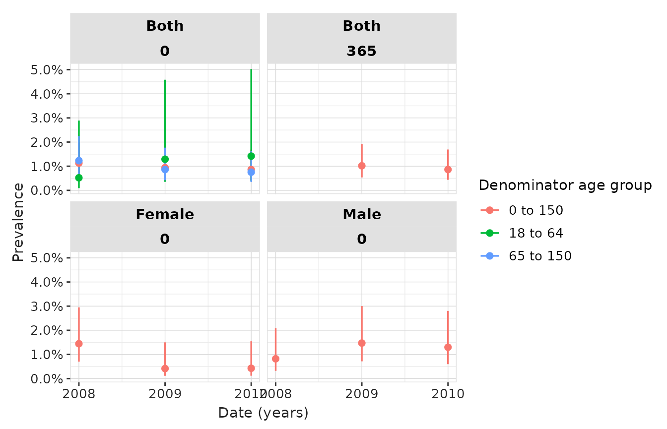

Prevalence

tablePrevalence(pop_diag,     
                groupColumn = c("cdm_name", "outcome_cohort_name"),
                hide = "denominator_cohort_name",
                settingsColumn = c("denominator_age_group",
                                   "denominator_sex",
                                   "denominator_days_prior_observation",
                                   "outcome_cohort_name"))

Prevalence start date	Prevalence end date	Analysis interval	Denominator age group	Denominator sex	Denominator days prior observation	Estimate name
Prevalence start date	Prevalence end date	Analysis interval	Denominator age group	Denominator sex	Denominator days prior observation	Denominator (N)	Outcome (N)	Prevalence [95% CI]
synpuf-1k; ankle_sprain
2008-01-01	2008-12-31	years	0 to 150	Both	0	973	11	0.01 (0.01 - 0.02)
2009-01-01	2009-12-31	years	0 to 150	Both	0	958	9	0.01 (0.00 - 0.02)
2010-01-01	2010-12-31	years	0 to 150	Both	0	930	8	0.01 (0.00 - 0.02)
2008-01-01	2010-12-31	overall	0 to 150	Both	0	1,000	27	0.03 (0.02 - 0.04)
2009-01-01	2009-12-31	years	0 to 150	Both	365	885	9	0.01 (0.01 - 0.02)
2010-01-01	2010-12-31	years	0 to 150	Both	365	928	8	0.01 (0.00 - 0.02)
2008-12-31	2010-12-31	overall	0 to 150	Both	365	979	17	0.02 (0.01 - 0.03)
2008-01-01	2008-12-31	years	0 to 150	Female	0	485	7	0.01 (0.01 - 0.03)
2009-01-01	2009-12-31	years	0 to 150	Female	0	482	2	0.00 (0.00 - 0.01)
2010-01-01	2010-12-31	years	0 to 150	Female	0	468	2	0.00 (0.00 - 0.02)
2008-01-01	2010-12-31	overall	0 to 150	Female	0	498	11	0.02 (0.01 - 0.04)
	2008-12-31	years	0 to 150	Male	0	488	4	0.01 (0.00 - 0.02)
2009-01-01	2009-12-31	years	0 to 150	Male	0	476	7	0.01 (0.01 - 0.03)
2010-01-01	2010-12-31	years	0 to 150	Male	0	462	6	0.01 (0.01 - 0.03)
2008-01-01	2010-12-31	overall	0 to 150	Male	0	502	16	0.03 (0.02 - 0.05)
	2008-12-31	years	18 to 64	Both	0	192	1	0.01 (0.00 - 0.03)
2009-01-01	2009-12-31	years	18 to 64	Both	0	155	2	0.01 (0.00 - 0.05)
2010-01-01	2010-12-31	years	18 to 64	Both	0	141	2	0.01 (0.00 - 0.05)
2008-01-01	2010-12-31	overall	18 to 64	Both	0	200	5	0.03 (0.01 - 0.06)
	2008-12-31	years	65 to 150	Both	0	813	10	0.01 (0.01 - 0.02)
2009-01-01	2009-12-31	years	65 to 150	Both	0	812	7	0.01 (0.00 - 0.02)
2010-01-01	2010-12-31	years	65 to 150	Both	0	797	6	0.01 (0.00 - 0.02)
2008-01-01	2010-12-31	overall	65 to 150	Both	0	855	22	0.03 (0.02 - 0.04)

results <- pop_diag |> 
  omopgenerics::filterSettings(result_type == "prevalence") |>
  visOmopResults::filterAdditional(analysis_interval == "years")
plotPrevalence(results,
               colour = "denominator_age_group",
               facet = c("denominator_sex", "denominator_days_prior_observation"))