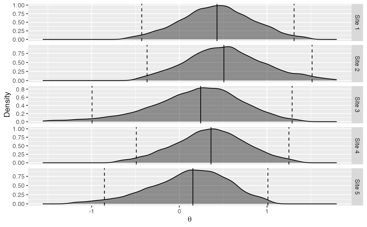
Plot posterior density per database

Plot posterior density per database

plotPerDbPosterior(
  estimate,
  showEstimate = TRUE,
  dataCutoff = 0.01,
  fileName = NULL
)

Arguments

estimate

An object as generated using the computeBayesianMetaAnalysis() function.

showEstimate

Show the parameter estimates (mode) and 95 percent confidence intervals?

dataCutoff

This fraction of the data at both tails will be removed.

fileName

Name of the file where the plot should be saved, for example 'plot.png'. See the function ggplot2::ggsave in the ggplot2 package for supported file formats.

Value

A Ggplot object. Use the ggplot2::ggsave function to save to file.

Details

Plot the density of the posterior distribution of the theta parameter (the estimated log hazard ratio) at each site.

Examples

# Simulate some data for this example:
populations <- simulatePopulations()

# Fit a Cox regression at each data site, and approximate likelihood function:
fitModelInDatabase <- function(population) {
  cyclopsData <- Cyclops::createCyclopsData(Surv(time, y) ~ x + strata(stratumId),
    data = population,
    modelType = "cox"
  )
  cyclopsFit <- Cyclops::fitCyclopsModel(cyclopsData)
  approximation <- approximateLikelihood(cyclopsFit, parameter = "x", approximation = "custom")
  return(approximation)
}
approximations <- lapply(populations, fitModelInDatabase)
approximations <- do.call("rbind", approximations)

# At study coordinating center, perform meta-analysis using per-site approximations:
estimate <- computeBayesianMetaAnalysis(approximations)
#> Detected data following custom parameric distribution
#> Performing MCMC. This may take a while
plotPerDbPosterior(estimate)