Step 1. Generate a sequence cohort • CohortSymmetry

Introduction

In this vignette we will explore the functionalities of generateSequenceCohort().

Create a cdm object

CohortSymmetry package is designed to work with data mapped to OMOP, so the first step is to create a reference to the data using the CDMConnector package. We will use the Eunomia dataset for the subsequent examples.

library(CDMConnector)
library(dplyr)
library(DBI)
library(CohortSymmetry)
library(duckdb)

db <- DBI::dbConnect(duckdb::duckdb(), 
                     dbdir = CDMConnector::eunomia_dir())
cdm <- cdm_from_con(
  con = db,
  cdm_schema = "main",
  write_schema = "main"
)

Instantiate two cohorts in the cdm reference

CohortSymmetry package requires that the cdm object contains two cohort tables: the index cohort and the marker cohort. There are a lot of different ways to create these cohorts, and it will depend on what the index cohort and marker cohort represent. Here, we use the DrugUtilisation package to generate two drug cohorts in the cdm object. For illustrative purposes, we will carry out SSA on aspirin (index_cohort) against acetaminophen (marker_cohort).

library(DrugUtilisation)
cdm <- DrugUtilisation::generateIngredientCohortSet(
  cdm = cdm,
  name = "aspirin",
  ingredient = "aspirin")

cdm <- DrugUtilisation::generateIngredientCohortSet(
  cdm = cdm,
  name = "acetaminophen",
  ingredient = "acetaminophen")

Generate a sequence cohort

In order to initiate the calculations, the two cohorts tables need to be intersected using generateSequenceCohortSet(). This process will output all the individuals who appear on both tables subject to different parameters. Each parameter corresponds to a specific requirement. The parameters for this function include cohortDateRange, daysPriorObservation, washoutWindow, indexMarkerGap and combinationWindow. Let’s go through examples to see how each parameter works.

No specific requirements

Let’s study the simplest case where no requirements are imposed. See figure below to see an example of an analysis containing six different participants.

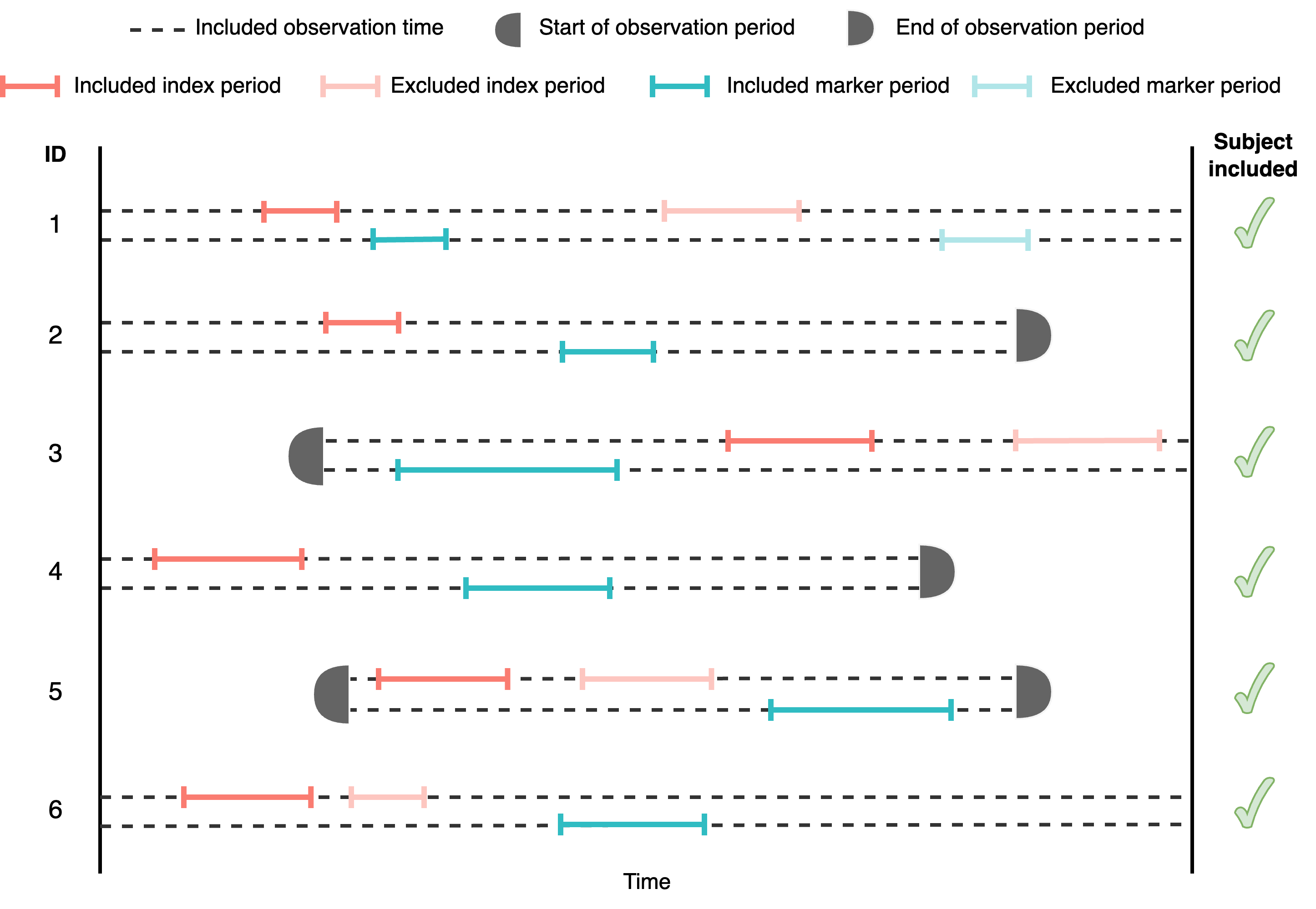
See that only the first event/episode (for both the index and the marker) is included in the analysis. As there is no restriction criteria and all the individuals have an episode in the index and the marker cohort, all the subjects are included in the analysis. We can get a sequence cohort without including any particular requirement like so:

cdm <- generateSequenceCohortSet(
  cdm = cdm,
  indexTable = "aspirin",
  markerTable = "acetaminophen",
  name = "intersect",
  cohortDateRange = as.Date(c(NA, NA)), #default
  daysPriorObservation = 0, #default
  washoutWindow = 0, #default
  indexMarkerGap = Inf, #default
  combinationWindow = c(0,Inf)) # default

cdm$intersect |> 
  dplyr::glimpse()
#> Rows: ??
#> Columns: 6
#> Database: DuckDB v1.1.3-dev165 [unknown@Linux 6.5.0-1025-azure:R 4.4.2//tmp/RtmpvJDqex/file17c470eaac46.duckdb]
#> $ cohort_definition_id <int> 1, 1, 1, 1, 1, 1, 1, 1, 1, 1, 1, 1, 1, 1, 1, 1, 1…
#> $ subject_id           <int> 42, 35, 2, 49, 11, 43, 12, 7, 17, 5, 30, 3, 57, 1…
#> $ cohort_start_date    <date> 1914-07-09, 1960-06-20, 1920-07-01, 1976-11-13, …
#> $ cohort_end_date      <date> 1937-09-07, 1993-04-28, 1931-09-03, 1978-03-10, …
#> $ index_date           <date> 1914-07-09, 1993-04-28, 1920-07-01, 1976-11-13, …
#> $ marker_date          <date> 1937-09-07, 1960-06-20, 1931-09-03, 1978-03-10, …

Important Observations

See that the generated table has the format of an OMOP CDM cohort, but it also includes two additional columns: the index_date and the marker_date, which are the cohort_start_date of the index and marker episode respectively. The cohort_start_date and the cohort_end_date are defined as:

cohort_start_date: earliest cohort_start_date between the index and the marker events.
cohort_end_date: latest cohort_start_date between the index and the marker events.

The cohort_definition_id in the output is associated with the cohort_definition_id} of the index table (indexId) and the cohort_definition_id of the marker table (markerId). To see the correspondence, one could do the following:

attr(cdm$intersect, "cohort_set")
#> # Source:   table<main.intersect_set> [1 x 13]
#> # Database: DuckDB v1.1.3-dev165 [unknown@Linux 6.5.0-1025-azure:R 4.4.2//tmp/RtmpvJDqex/file17c470eaac46.duckdb]
#>   cohort_definition_id cohort_name     index_id index_name marker_id marker_name
#>                  <int> <chr>              <int> <chr>          <int> <chr>      
#> 1                    1 index_1191_asp…        1 1191_aspi…         1 161_acetam…
#> # ℹ 7 more variables: cohort_date_range <chr>, days_prior_observation <chr>,
#> #   washout_window <chr>, index_marker_gap <chr>, combination_window <chr>,
#> #   moving_average_restriction <chr>, nsr <dbl>

The user may also wish to subset the index table and marker table based on their cohort_definition_id using indexId and markerId respectively. For example, the following code only includes cohort_definidtion_id $= 1$ from both the index and the marker table.

cdm <- generateSequenceCohortSet(
  cdm = cdm,
  indexTable = "aspirin",
  markerTable = "acetaminophen",
  name = "intersect",
  cohortDateRange = as.Date(c(NA, NA)),
  indexId = 1,
  markerId = 1,
  daysPriorObservation = 0,
  washoutWindow = 0,
  indexMarkerGap = NULL,
  combinationWindow = c(0,Inf))

Specified study period

We can restrict the study period of the analysis to only include episodes or events happening during a specific period of time. See figure below to see an example of an analysis containing six different participants.

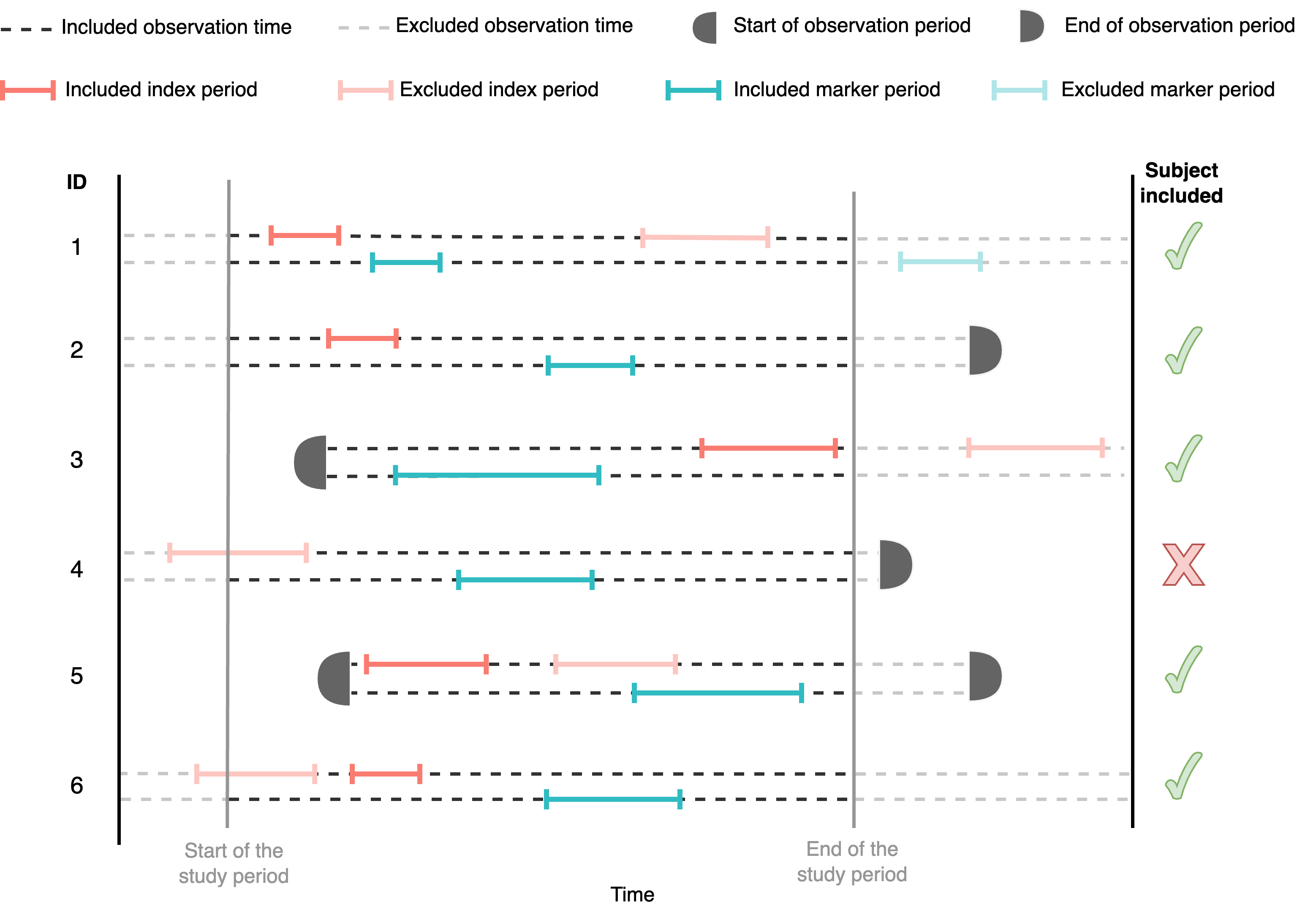
Notice that, by imposing a restriction on study period, some of the participants might be excluded. For example, participant 4 is excluded because the only index episode is outside of the study period whereas participant 6 is included because he/she does have an index episode within the study period.

The study period can be restricted using the cohortDateRange argument, which is defined as:

cohortDateRange = c(start_of_the_study_period, end_of_the_study_period)

See an example of the usage below, where we have restricted the cohortDateRange within 01/01/1950 until 01/01/1969.

cdm <- generateSequenceCohortSet(
  cdm = cdm,
  indexTable = "aspirin",
  markerTable = "acetaminophen",
  name = "intersect_study_period",
  cohortDateRange = as.Date(c("1950-01-01","1969-01-01")))

Specified study period and prior history requirement

We can also specify the minimum prior history that an individual has to have before the start of the first event. Individuals with not enough prior history will be excluded. See the figure below, imagine the prior observation history is set to be 31 days, then participant 5 would be excluded because the first event happening within the study period does not have more than (or equal to) 31 days of prior history:

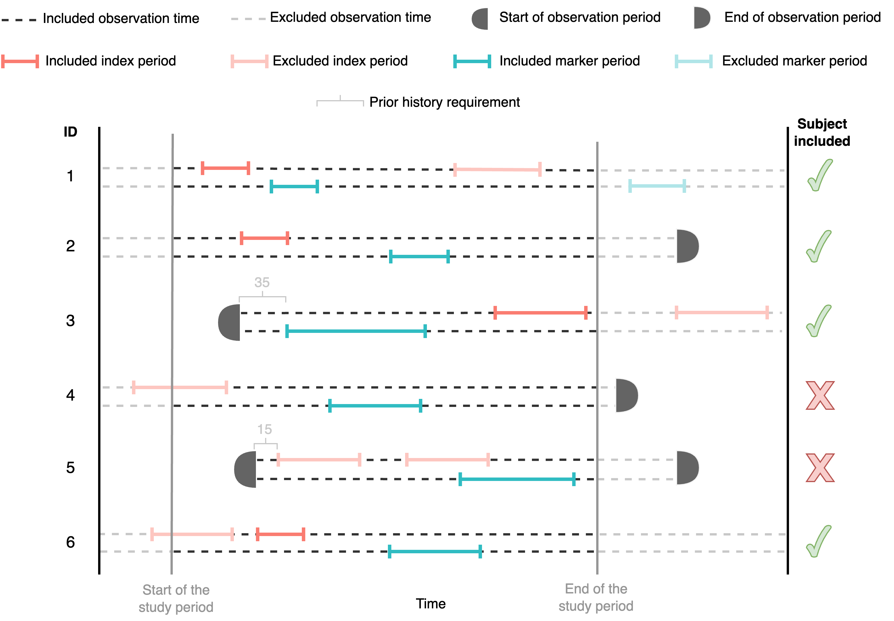
The number of days of prior history required can be implemented using the argument daysPriorObservation. See an example below:

 cdm <- generateSequenceCohortSet(
   cdm = cdm,
   indexTable = "aspirin",
   markerTable = "acetaminophen",
   name = "intersect_prior_obs",
   cohortDateRange = as.Date(c("1950-01-01","1969-01-01")),
   daysPriorObservation = 365)

Specified study period, prior history requirement and washout period

We can also specify the minimum washout period required for an event or episode to be included. In the following figure, we exclude participant 6 as another episode took place within the washout period. Washout period is applied to index and marker respectively.

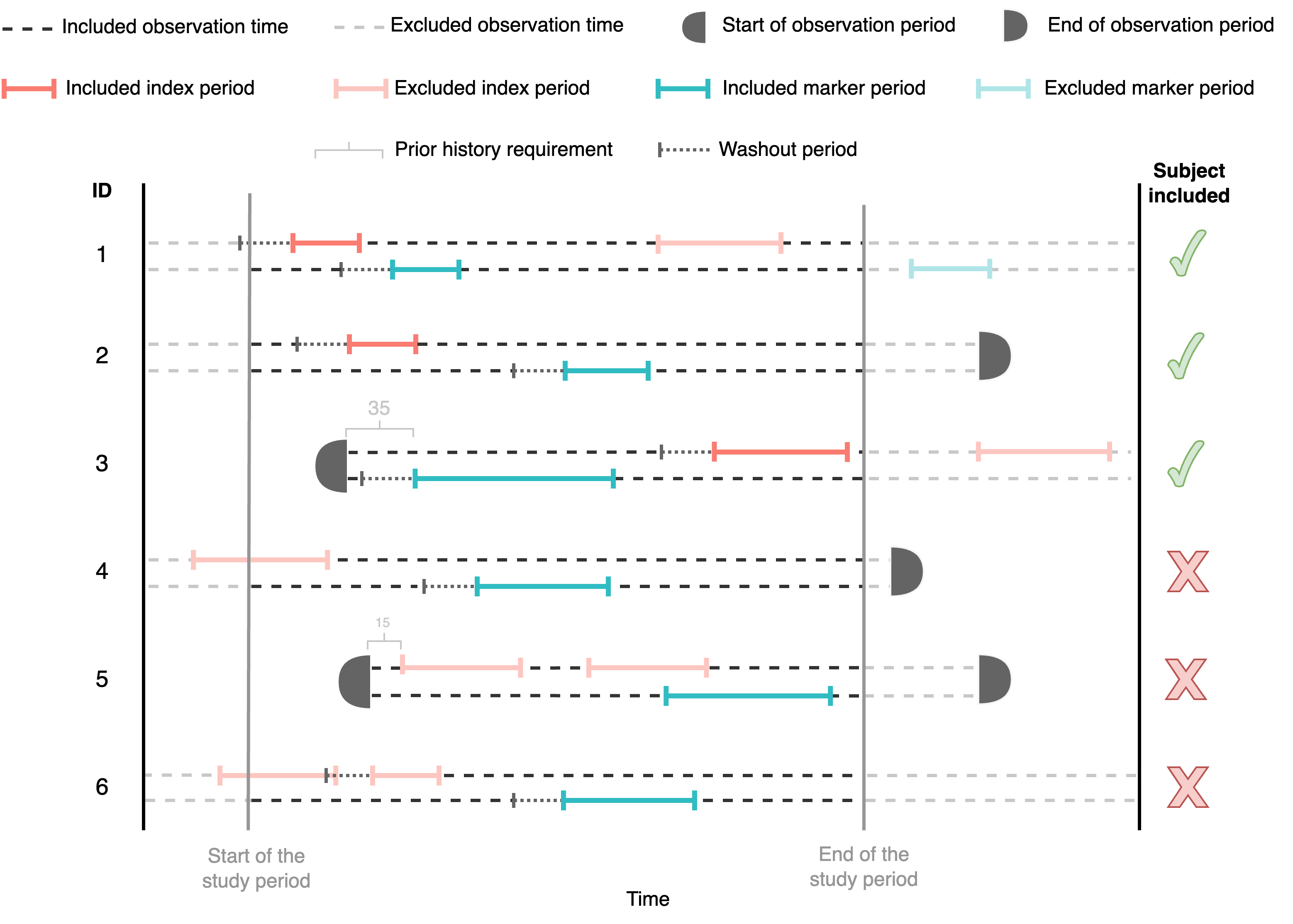
This functionality can be implemented using the washoutWindow argument. See an example below:

cdm <- generateSequenceCohortSet(
  cdm = cdm,
  indexTable = "aspirin",
  markerTable = "acetaminophen",
  name = "intersect_washout",
  cohortDateRange = as.Date(c("1950-01-01","1969-01-01")),
  daysPriorObservation = 365,
  washoutWindow = 365)

Specified study period, prior history requirement and combination window

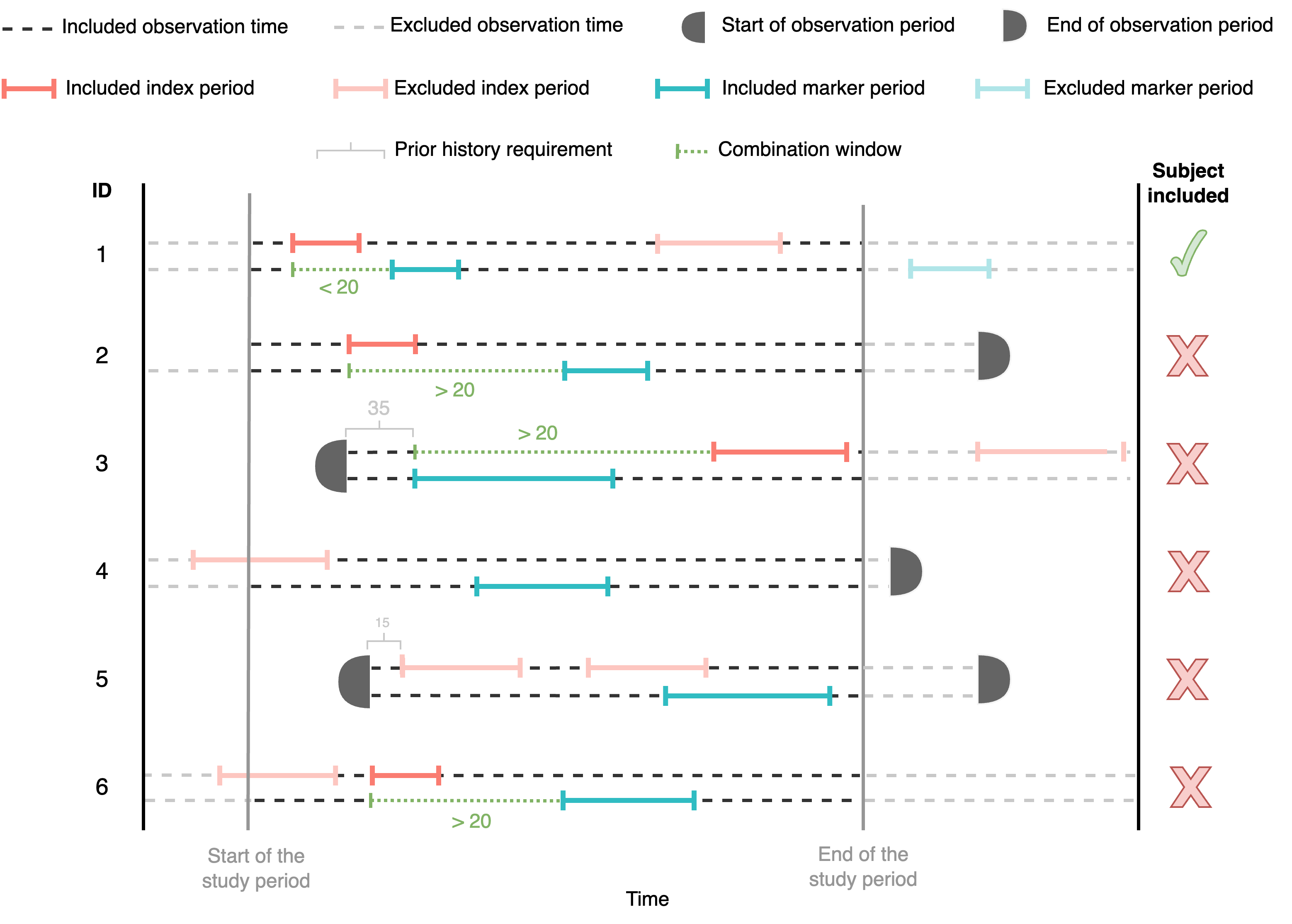
We define the combination window as the minimum and the maximum days between the start of the first event (either if is the index or the marker) and the start of the next event. In other words:

$x =$ second_episode(start_date) $-$ first_episode(start_date);

combinationWindow[1] $< x \leq$ combinationWindow[2]

See in the figure below an example, where we define combinationWindow = c(0,20). This means that the gap between the start date of the second episode and the start of the first episode should be larger than 0 and less or equal than 20. As participant 2 and 3 do not fulfill this condition, they are excluded from the analysis.

In the generateSequenceCohortSet() function, this is implemented using the combinationWindow argument. Notice that in the previous examples, as we did not want any combination window requirement, we have set this argument to combinationWindow = c(0,Inf), as by default is combinationWindow = c(0, 365). In the following example, we explore subject_id 80 and 187 to see the functionality of this argument. When using no restriction for the combination window, both are included in the intersect_changed_cw cohort:

 cdm <- generateSequenceCohortSet(
   cdm = cdm,
   indexTable = "aspirin",
   markerTable = "acetaminophen",
   name = "intersect_changed_cw",
   cohortDateRange = as.Date(c("1950-01-01","1969-01-01")),
   daysPriorObservation = 365,
   combinationWindow = c(0, Inf))

 cdm$intersect_changed_cw |>
   dplyr::filter(subject_id %in% c(80,187)) |>
   dplyr::mutate(combinationWindow = pmax(index_date, marker_date) - pmin(index_date, marker_date))

Specified study period, prior history requirement and index marker gap

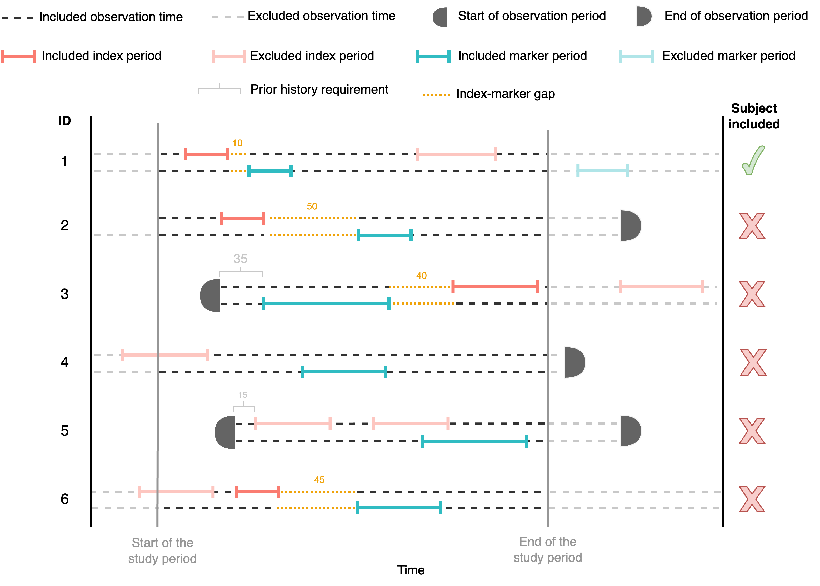
We define the index-marker gap to refer to the maximum number of days between the start of the second episode and the end of the first episode. That means:

$x =$ second_episode(cohort_start_date) $-$ first_episode(cohort_end_date);

x $\leq$ indexMarkerGap

See an example below, where all participants with an index-marker gap higher than 30 days are excluded from the analysis (participant 2, 3 and 6):

Use indexGap argument to impose this restriction, for example:

cdm <- generateSequenceCohortSet(
  cdm = cdm,
  indexTable = "aspirin",
  markerTable = "acetaminophen",
  name = "intersect_",
  cohortDateRange = as.Date(c("1950-01-01","1969-01-01")),
  daysPriorObservation = 365,
  indexMarkerGap = 7)

CDMConnector::cdmDisconnect(cdm = cdm)