The goal of CohortSymmetry is to carry out the necessary calculations for Sequence Symmetry Analysis (SSA). It is highly recommended that this method is tested beforehand against well-known positive and negative controls. Such controls could be found using Pratt et al (2015).
Installation
You can install the development version of CohortSymmetry from GitHub with:
# install.packages("pak")
pak::pak("OHDSI/CohortSymmetry")
Example
Create a reference to data in the OMOP CDM format
The CohortSymmetry package is designed to work with data mapped to OMOP CDM, so the first step is to create a mock database using the omock package. We will use the Eunomia dataset within omock for the subsequent examples. There are other synthetic datasets within omock that users can also use to get familiar with CohortSymmetry before applying to their own database. See the omock vignette for more details.
As an example, we will be using Eunomia GIBleed data set.
library(dplyr)
library(DBI)
library(omock)
library(CohortSymmetry)

cdm <- mockCdmFromDataset(datasetName = "GiBleed")
Step 0: Instantiate two cohorts in the cdm reference
This will be entirely user’s choice on how to generate such cohorts. Minimally, this package requires two cohort tables in the cdm reference, namely the index_cohort and the marker_cohort.
If one wants to generate two drugs cohorts in cdm, the DrugUtilisation R package can be used or we recommend using CohortConstructor R package. However a user will need to specify the gap eras for each of the cohorts i.e. a gap era set to 30 would collapse episodes together if they are within 30 days of each other for example please see the individual packages on how to implement this if required.
For merely illustration purposes, we will carry out SSA on aspirin (index_cohort) against amoxicillin (marker_cohort). Multiple markers can be instantiated in the marker cohort and each one will be tested against the index cohort.
Using the drug utilisation package:
library(dplyr)
library(DrugUtilisation)

cdm <- DrugUtilisation::generateIngredientCohortSet(
  cdm = cdm,
  name = "aspirin",
  ingredient = "aspirin")
#> ℹ Subsetting drug_exposure table
#> ℹ Checking whether any record needs to be dropped.
#> ℹ Collapsing overlaping records.
#> ℹ Collapsing records with gapEra = 1 days.

cdm <- DrugUtilisation::generateIngredientCohortSet(
  cdm = cdm,
  name = "amoxicillin",
  ingredient = "amoxicillin")
#> ℹ Subsetting drug_exposure table
#> ℹ Checking whether any record needs to be dropped.
#> ℹ Collapsing overlaping records.
#> ℹ Collapsing records with gapEra = 1 days.
Using CohortConstructor R package (recommended):
library(dplyr)
library(CodelistGenerator)
library(CohortConstructor)

aspirin_codelist <- CodelistGenerator::getDrugIngredientCodes(
  cdm = cdm,
  name = "aspirin",
  nameStyle = "{concept_name}"
)

cdm[["aspirin"]] <- CohortConstructor::conceptCohort(
  cdm = cdm,
  conceptSet = aspirin_codelist,
  exit = "event_end_date",
  name = "aspirin")
#> ℹ Subsetting table drug_exposure using 2 concepts with domain: drug.
#> ℹ Combining tables.
#> ℹ Creating cohort attributes.
#> ℹ Applying cohort requirements.
#> ℹ Merging overlapping records.
#> ✔ Cohort aspirin created.


amoxicillin_codelist <- CodelistGenerator::getDrugIngredientCodes(
  cdm = cdm,
  name = "amoxicillin",
  nameStyle = "{concept_name}"
)

cdm[["amoxicillin"]] <- CohortConstructor::conceptCohort(
  cdm = cdm,
  conceptSet = amoxicillin_codelist,
  exit = "event_end_date",
  name = "amoxicillin")
#> ℹ Subsetting table drug_exposure using 4 concepts with domain: drug.
#> ℹ Combining tables.
#> ℹ Creating cohort attributes.
#> ℹ Applying cohort requirements.
#> ℹ Merging overlapping records.
#> ✔ Cohort amoxicillin created.
Step 1: generateSequenceCohortSet
In order to initiate the calculations, the two cohorts tables need to be intersected using generateSequenceCohortSet(). This process will output all the individuals who appeared on both tables according to a user-specified parameters. This includes cohortDateRange, combinationWindow, washoutWindow, indexMarkerGap and daysPriorObservation. More details on these parameters are found on the vignette.
library(CohortSymmetry)

cdm <- generateSequenceCohortSet(
  cdm = cdm,
  indexTable = "aspirin",
  markerTable = "amoxicillin",
  name = "aspirin_amoxicillin"
)

cdm$aspirin_amoxicillin %>%
  dplyr::glimpse()
#> Rows: 72
#> Columns: 6
#> $ cohort_definition_id <int> 1, 1, 1, 1, 1, 1, 1, 1, 1, 1, 1, 1, 1, 1, 1, 1, 1…
#> $ subject_id           <int> 1536, 1340, 2801, 4121, 4867, 1054, 2813, 331, 34…
#> $ cohort_start_date    <date> 1912-08-25, 1912-10-22, 1923-06-17, 1925-09-28, …
#> $ cohort_end_date      <date> 1913-01-27, 1912-12-29, 1923-11-09, 1925-11-18, …
#> $ index_date           <date> 1912-08-25, 1912-10-22, 1923-11-09, 1925-11-18, …
#> $ marker_date          <date> 1913-01-27, 1912-12-29, 1923-06-17, 1925-09-28, …
Step 2: summariseSequenceRatios
To get the sequence ratios, we would need the output of the generateSequenceCohortSet() function to be fed into summariseSequenceRatios() The output of this process contains CSR(crude sequence ratio), ASR(adjusted sequence ratio) and confidence intervals.
res <- summariseSequenceRatios(cohort = cdm$aspirin_amoxicillin)

res %>% glimpse()
#> Rows: 11
#> Columns: 13
#> $ result_id        <int> 1, 1, 1, 1, 1, 1, 1, 1, 1, 1, 1
#> $ cdm_name         <chr> "GiBleed", "GiBleed", "GiBleed", "GiBleed", "GiBleed"…
#> $ group_name       <chr> "index_cohort_name &&& marker_cohort_name", "index_co…
#> $ group_level      <chr> "aspirin &&& amoxicillin", "aspirin &&& amoxicillin",…
#> $ strata_name      <chr> "overall", "overall", "overall", "overall", "overall"…
#> $ strata_level     <chr> "overall", "overall", "overall", "overall", "overall"…
#> $ variable_name    <chr> "index", "index", "marker", "marker", "null", "crude"…
#> $ variable_level   <chr> "first_pharmac", "first_pharmac", "first_pharmac", "f…
#> $ estimate_name    <chr> "count", "percentage", "count", "percentage", "point_…
#> $ estimate_type    <chr> "integer", "numeric", "integer", "numeric", "numeric"…
#> $ estimate_value   <chr> "42", "58.3", "30", "41.7", "1.04487150121398", "1.4"…
#> $ additional_name  <chr> "overall", "overall", "overall", "overall", "overall"…
#> $ additional_level <chr> "overall", "overall", "overall", "overall", "overall"…
Step 3: visualise the results
The user could then visualise their results using a wide array of provided tools.
For example, the following produces a gt table. This table contains the CSR, ASR and confidence intervals as well as the Null Sequence Ratio (NSR). It also contains the counts and percentages of how many sequences had the index first or marker first.
gt_results <- tableSequenceRatios(result = res)

gt_results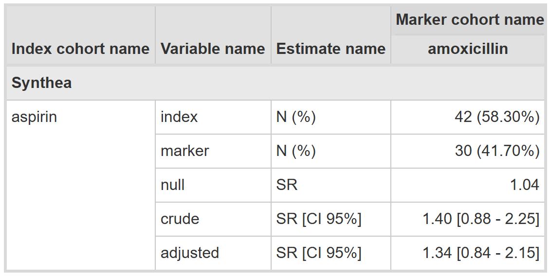
Note that flextable is also an option, users may specify this by using the type argument.
One could also visualise the plot, for example, the following is the plot of the crude and adjusted sequence ratio. There is flexibility to just show the ASR and update colours.
sequence_ratio_plot <- plotSequenceRatios(
  result = res,
  onlyASR = FALSE
)

sequence_ratio_plot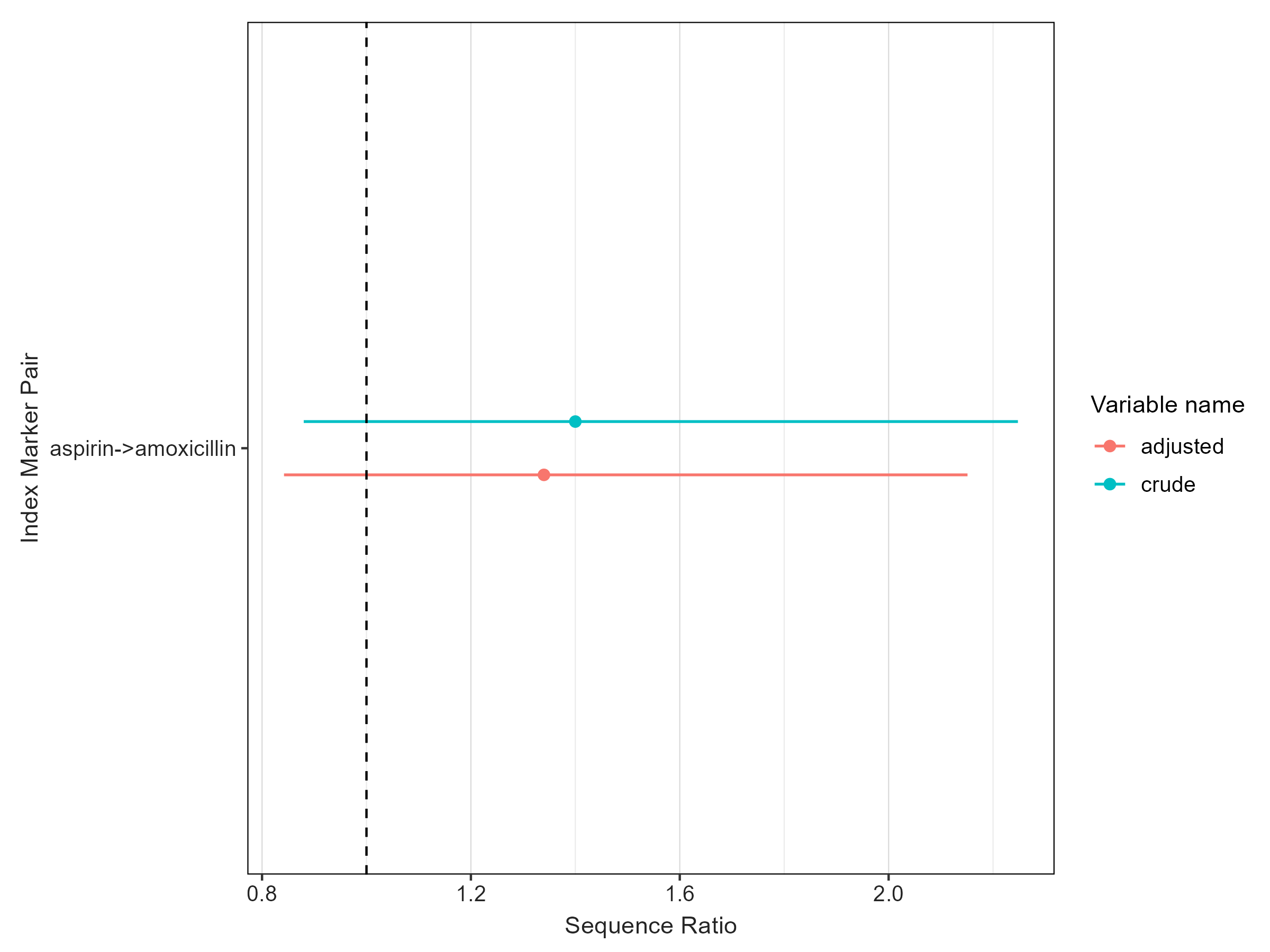
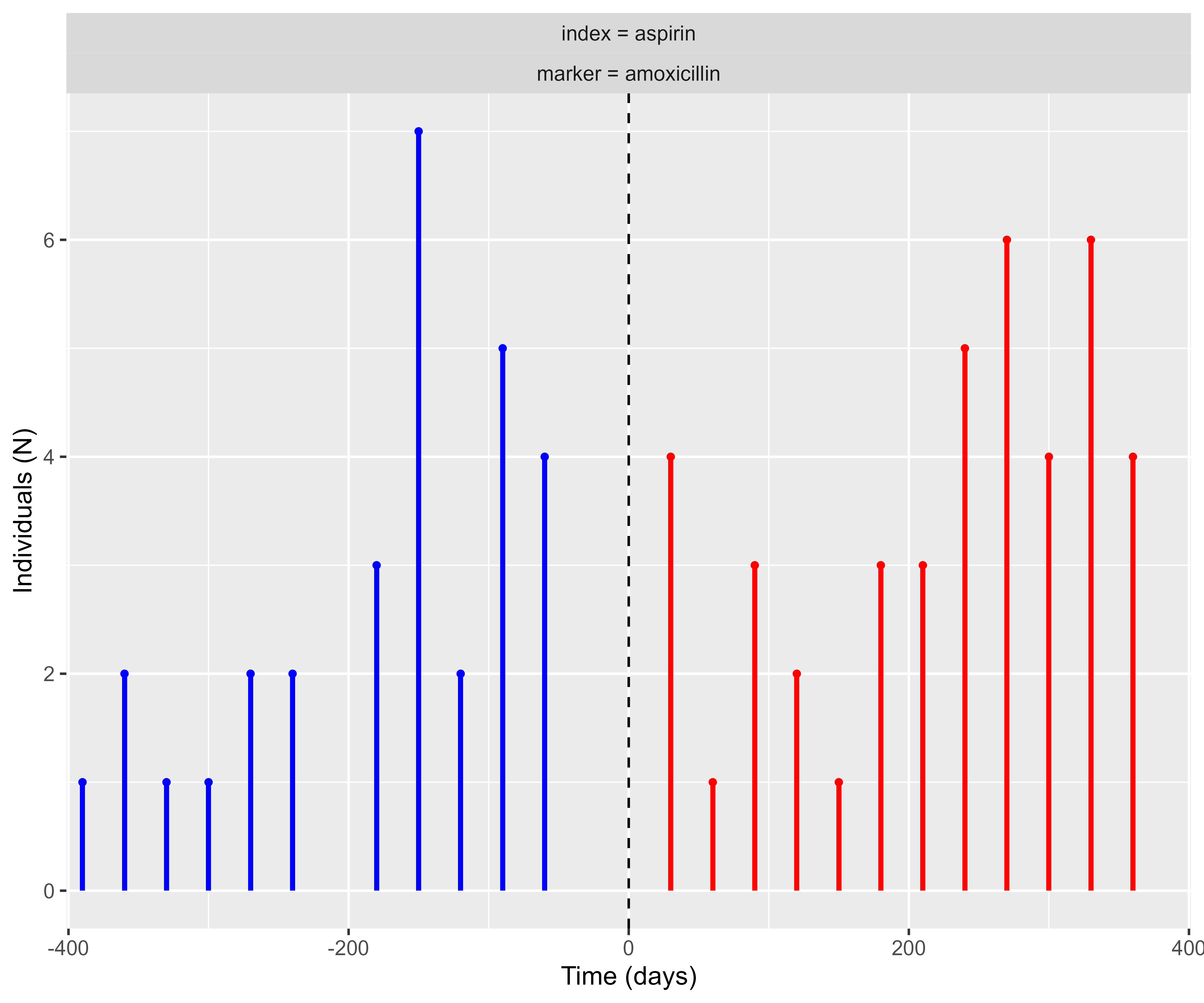
The user also has the freedom to plot temporal trend to review the asymmetry between index and marker. The argument days (default 30 days) allows the user to create specific breaks for this plot:
temporal_symmetry <- summariseTemporalSymmetry(cohort = cdm$aspirin_amoxicillin)

temporal_symmetry_plot <- plotTemporalSymmetry(
  result = temporal_symmetry
)

temporal_symmetry_plot