Introduction to CohortSymmetry

CohortSymmetry provides tools to perform Sequence Symmetry Analysis (SSA). Before using the package, it is highly recommended that this method is tested beforehand against well-known positive and negative controls. The details of SSA and the relevant controls could be found using Pratt et al (2015).

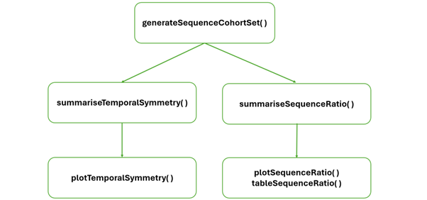
The functions you will interact with are:

1. generateSequenceCohortSet(): this function will create a cohort with individuals present in both (the index and the marker) cohorts.

2. summariseSequenceRatios(): this function will calculate sequence ratios.

3. tableSequenceRatios() and plotSequenceRatios(): these functions will help us to visualise the sequence ratio results.

4. summariseTemporalSymmetry(): this function will produce aggregated results based on the time difference between two cohort start dates.

5. plotTemporalSymmetry(): this function will help us to visualise the results from summariseTemporalSymmetry().

Below, you will find an example analysis that offers a brief and comprehensive overview of the package’s functionalities. More context and further examples for each of these functions are provided in later vignettes.

First, let’s load the relevant libraries.

library(omock)
library(CohortSymmetry)
library(visOmopResults)
library(dplyr)

The CohortSymmetry package works with data mapped to the OMOP CDM. Hence, the initial step involves connecting to a database which is user and database specific. As an example, we will be using omock package which can call various synthetic databases. We will use the GIBleed data to create two cohorts: the index_cohort and the marker_cohort.

cdm <- mockCdmFromDataset(datasetName = "GiBleed")

cdm <- DrugUtilisation::generateIngredientCohortSet(
  cdm = cdm, 
  name = "index",
  ingredient = "aspirin")

cdm <- DrugUtilisation::generateIngredientCohortSet(
  cdm = cdm,
  name = "marker",
  ingredient = c("amoxicillin"))

Once we have our data and created the index and marker cohorts, we can use the generateSequenceCohortSet() function to find the intersection of the two cohorts. This function will provide us with the individuals who appear in both cohorts, which will be named intersect - another cohort in the cdm reference.

cdm <- generateSequenceCohortSet(
  cdm = cdm,
  indexTable = "index",
  markerTable = "marker",
  name = "intersect",
  combinationWindow = c(0, 365)
)

See below that the generated cohort follows the format of an OMOP CDM cohort with the addition of two extra columns: index_date and marker_date. These columns correspond to the cohort_start_date in the index_cohort and the marker_cohort, respectively.

cdm$intersect |> 
  dplyr::glimpse()
#> Rows: 72
#> Columns: 6
#> $ cohort_definition_id <int> 1, 1, 1, 1, 1, 1, 1, 1, 1, 1, 1, 1, 1, 1, 1, 1, 1…
#> $ subject_id           <int> 1536, 1340, 2801, 4121, 4867, 1054, 2813, 331, 34…
#> $ cohort_start_date    <date> 1912-08-25, 1912-10-22, 1923-06-17, 1925-09-28, …
#> $ cohort_end_date      <date> 1913-01-27, 1912-12-29, 1923-11-09, 1925-11-18, …
#> $ index_date           <date> 1912-08-25, 1912-10-22, 1923-11-09, 1925-11-18, …
#> $ marker_date          <date> 1913-01-27, 1912-12-29, 1923-06-17, 1925-09-28, …

Once we have the intersect cohort, you are able to explore the temporal symmetry by using summariseTemporalSymmetry, tableTemporalSymmetry, and plotTemporalSymmetry():

temporal_symmetry <- summariseTemporalSymmetry(
  cohort = cdm$intersect, 
  days = 30)

The result can be viewed using table and plot functions.

tableTemporalSymmetry(result = temporal_symmetry)

Marker name	Estimate name	Variable level
		-390	-360	-330	-300	-270	-240	-180	-150	-120	-90	-60	30	60	90	120	150	180	210	240	270	300	330	360
GiBleed; aspirin
amoxicillin	30_days_ly_count	1	2	1	1	2	2	3	7	2	5	4	4	1	3	2	1	3	3	5	6	4	6	4

plotTemporalSymmetry(result = temporal_symmetry)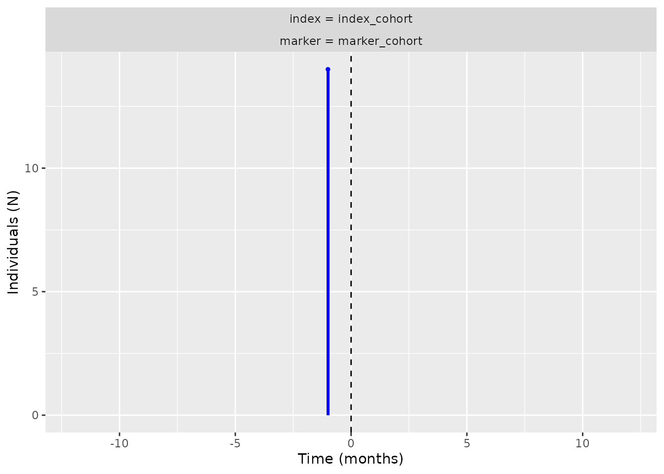

Next, we will use the summariseSequenceRatios() function to get the crude sequence ratios, adjusted sequence ratios, and the corresponding confidence intervals.

sequence_ratio <- summariseSequenceRatios(cohort = cdm$intersect)

Finally, we can visualise the results using tableSequenceRatios():

tableSequenceRatios(result = sequence_ratio)

Index cohort name	Variable name	Estimate name	Marker cohort name
			amoxicillin
GiBleed
aspirin	index	N (%)	42 (58.30%)
	marker	N (%)	30 (41.70%)
	null	SR	1.04
	crude	SR [CI 95%]	1.40 [0.88 - 2.25]
	adjusted	SR [CI 95%]	1.34 [0.84 - 2.15]

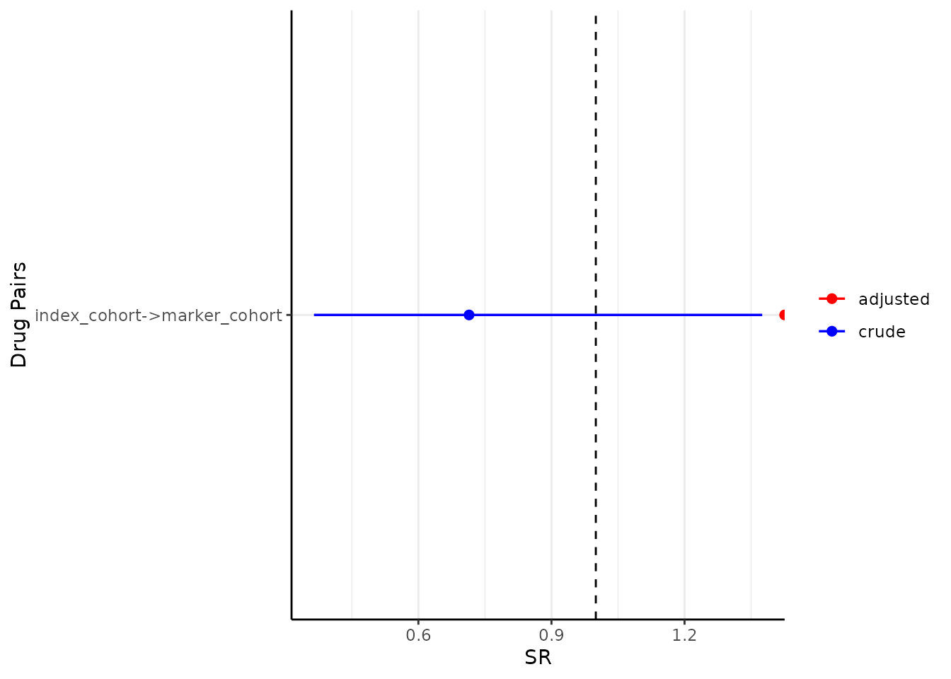
Or create a plot with the adjusted sequence ratios:

plotSequenceRatios(result = sequence_ratio)

As a diagram

Diagrammatically, the work flow using CohortSymmetry resembles the following flow chat: