 OHDSI GIS
 OHDSI GIS
WG
Examples
Worked examples of what you can do with the Gaia toolchain. Each one states the question, the data, what Gaia does with it, and what you learn, and links to the materials to run it yourself. The examples use synthetic persons (no real individuals, addresses or coordinates) together with real or simulated place data, so every result can be checked against a known answer.
1. Long-term PM2.5 and COPD
Question. Does long-term exposure to fine particulate matter relate to COPD?
Data. 10,000 synthetic adults placed at random points in real US counties, with residence histories (about 10% move once), 14 respiratory and cardiometabolic conditions and county-level social indicators. The exposure is real: monthly county PM2.5 from the CDC, 2014-2019. A simulated county SES index confounds the association.
What Gaia does.
- Describe the PM2.5 source in a catalog entry and judge its fitness for the question
- Ingest it and join it to the persons’ residences: where (the residence point falls inside a county polygon) and when (each monthly value is clipped to the residence interval)
- Land the result in the OMOP
EXTERNAL_EXPOSUREtable with standard concepts - Build exposure features and cohorts, and estimate the effect with HADES tools
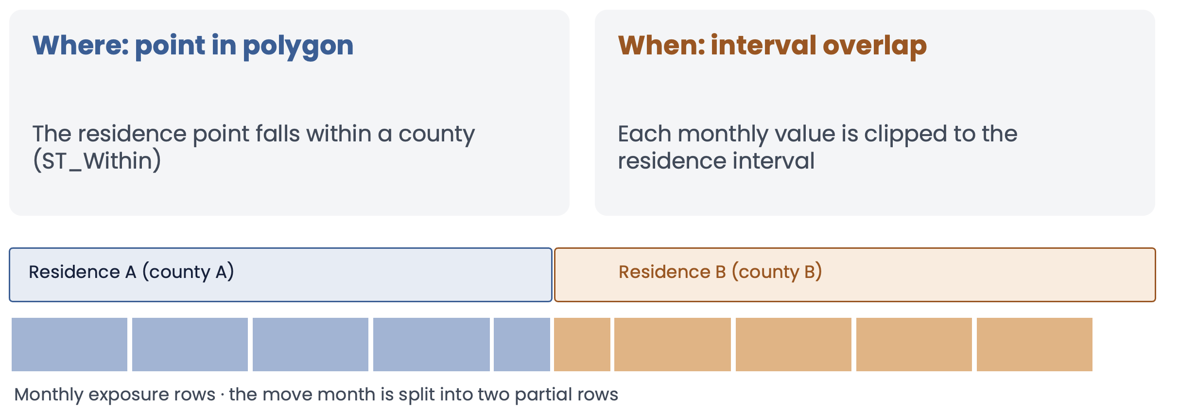
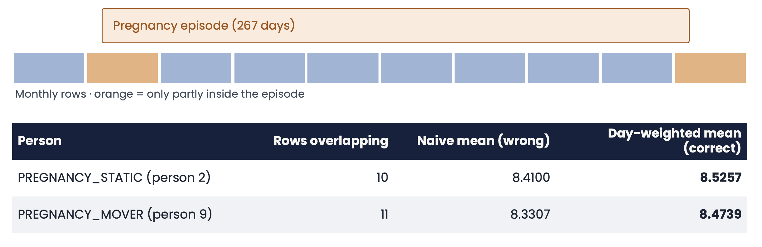
What you learn. The exposure of a person who moves is the day-weighted mean over both residences, and a naive mean of the monthly rows is wrong:
Logistic regression of COPD on the 24-month day-weighted PM2.5 recovers a slope of about 0.11 per µg/m³ after adjustment (the simulated truth is 0.15), and the negative-control outcome (CKD) is about 0 once SES is in the model. A high-versus-low CohortMethod comparison gives a COPD hazard ratio of about 1.26 (1.01 to 1.57) and about 0.94 for CKD. The simulated effects are deliberately exaggerated: they are a teaching device, not real-world estimates.
Run it. Tutorial, with the SQL and R tracks, the synthetic data description and the answer key.
2. Particle exposure by floor of a tall building
Question. If the exposure changes with the floor you live on, how much does it matter when the floor is not known exactly?
Data. A synthetic 100-floor tower flattened to a row of 100 adjacent floor polygons (height is the x axis), with four particle sensors (points) on every floor, daily readings for a year, and 10,000 persons placed in different parts of the floors. PM2.5 rises with height by design (illustrative, not physical), and a person-level SES index that rises with the floor confounds the effect in the opposite direction to example 1.
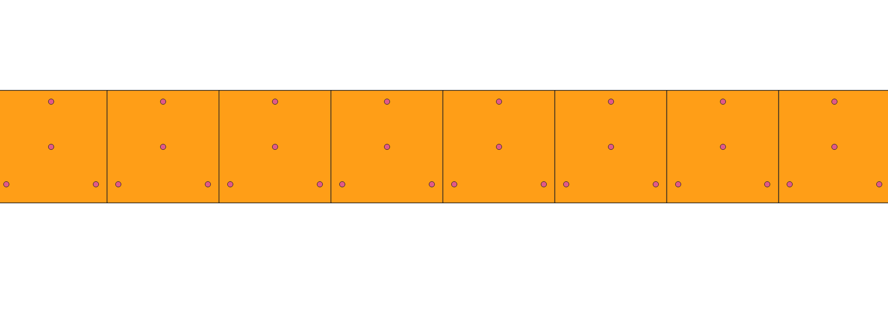
Eight floors in QGIS: each 30 m by 30 m floor is a polygon, with three sensors near the windows and one at the core.
What Gaia does. The sensors become a point source and the floors a polygon source in the catalog. Each person’s exposure is the floor mean of the sensors, joined by point-in-polygon and clipped to the residence interval, 365 daily rows per person and 3.65 million rows in all. They match an independent answer key exactly.
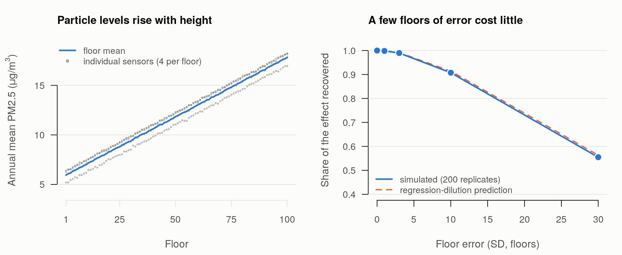
What you learn. A 2D geocoder does not know the floor. Because the gradient is smooth, an error of a few floors costs almost nothing, and it takes errors of about 10 floors to lose 10% of the effect. The loss follows the regression-dilution prediction closely. Grouping floors into zones (a Berkson-type error) loses little, whereas a random floor loses all of it, and without SES in the model the effects are biased down and the null outcomes look protective (the “penthouse” confounding).
Run it. syntheticDataGIS/tower:
generator, catalog entries, a check of the Gaia join against the answer
key, and a loader that puts the floors, sensors and people in a running
gaia-db so you can look at them in QGIS.
3. Exposure from raster data: surfaces, annual layers and land cover
Question. When the exposure is a grid of cells rather than polygons or points, how should a person’s residence be linked to it: the value of the cell they live in, or a summary of the cells around them? And how do annual layers line up with a person who moves?
Data. Simulated rasters over a 10 km window around
downtown Los Angeles, with a known answer key and 500 test points. There
are three exposure surfaces (25 m, 250 m and 2.5 km cells) that are the
same fields as the vector
synthetic_surface_* grids, so raster and vector can be
compared cell for cell. There is also a six-year series (2014 to 2019,
one file per year, with a trend that grows from west to east and a small
nodata hole) and a land cover layer with four classes. None of it
measures a real exposure.
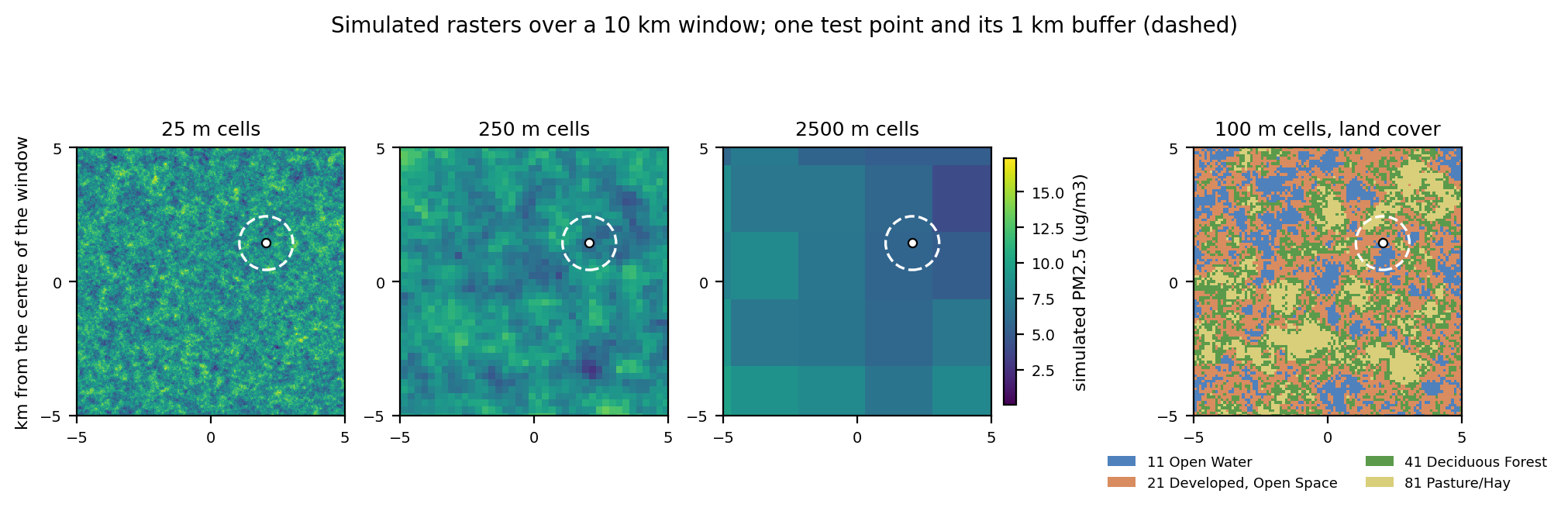
The surfaces are one random field at three cell sizes (25 m, 250 m and 2.5 km), shown with the 100 m land cover. The dashed circle is a 1 km buffer around one test point: the join returns the value of the cell under the point, the mean of the cells in the circle, or, for land cover, the share of each class.
What Gaia does. Each raster has a catalog entry
(structure: raster). ingest_datasource
downloads the file, loads it with raster2pgsql and
registers its variables and layers, so each layer knows the period it
stands for. A residence is then joined three ways: by the cell
value at the point, by the mean of the cells
within a radius, or, for land cover, by the share of each
class in a radius. As for vector sources, each annual layer is
clipped to the residence interval, so a person who moves in the middle
of a year gets two rows with the dates split at the move. The results
land in EXTERNAL_EXPOSURE.
What you learn. The cell value at the point matches the answer key exactly (500 rows per static layer and 2,964 for the annual series, with nodata giving no row), and the buffer means and class shares agree with it to within the small difference between a geography buffer in metres and a planar one. The cell value is not the true value at the point: with cells a quarter of the field’s correlation length, the two differ by about 0.65 µg/m³ on average at every scale, which is the price of using a raster. Because the exposure of someone who moves is built from the layers of both periods, the annual series shows why dates matter as much as locations. The design questions that remain open (relationship concepts, where class codes go, performance on large rasters) are in the raster discussion.
Run it. syntheticDataGIS/raster:
generator, answer key, catalog entries and a script that loads
everything into a throwaway gaia-db and compares the join with the key.
The functions are described under Raster Sources
in gaiaDB.
4. From monitors to people: Voronoi cells
Question. A network of monitors measures the exposure at a few points. How do you give a person who lives between them an exposure, and how many monitors does that take?
Data. Simulated PM2.5 monitors sampling a known exposure field over a 10 km window around downtown Los Angeles (the field of the raster example): nested networks of 20, 60 and 200 monitors, each reading the true field plus noise once a year for 2014 to 2019, and 500 synthetic persons who live at fixed points. Because the true exposure at every person is known, every way of assigning it can be scored. None of it measures a real exposure.
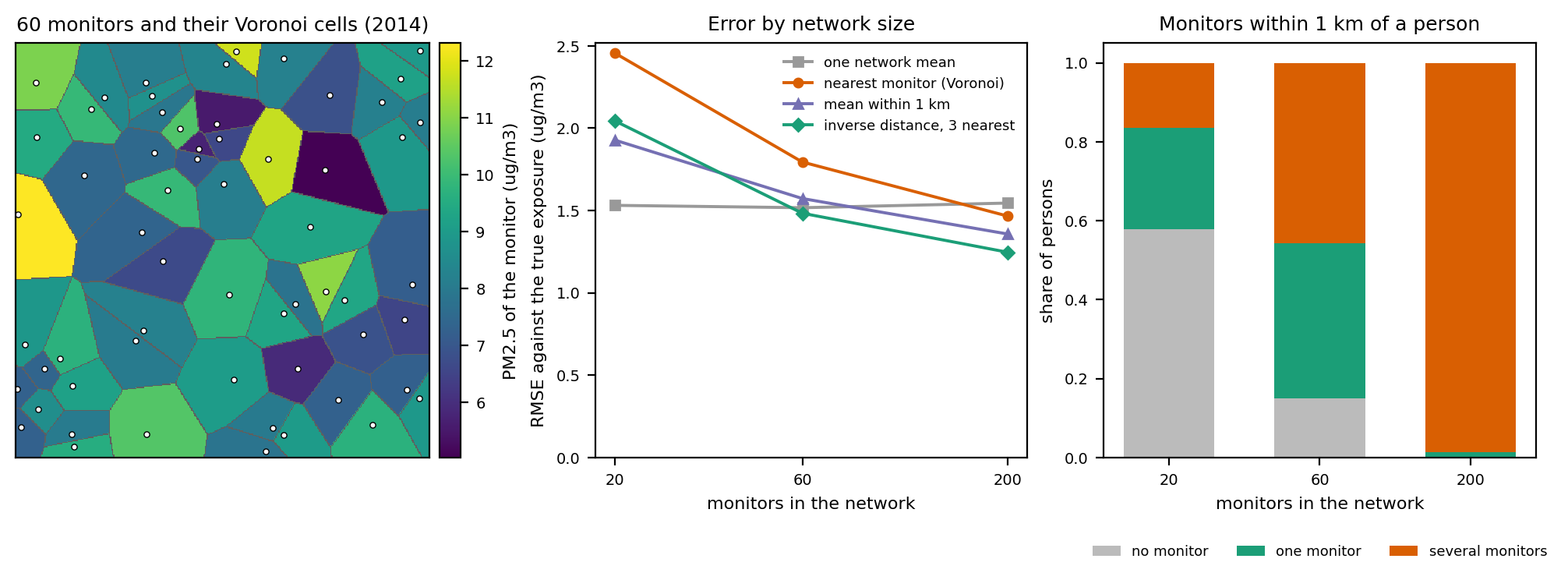
Left: the cells of a network of 60 monitors, coloured by the monitor’s reading (every location belongs to the cell of its nearest monitor). Middle: the error of four ways of assigning exposure against the true field. Right: what a 1 km buffer gives a person.
What Gaia does. The monitors are a point source in
the catalog. A second catalog entry holds their Voronoi
cells, built from the point source in the ETL step
(backbone.create_voronoi_source), which makes it a polygon
source that carries each monitor’s series. The cells then join to the
persons like any polygon source: where (the residence
falls inside a cell) and when (each annual value is
clipped to the residence interval), and the rows land in
EXTERNAL_EXPOSURE. For a point source that is not worth
tessellating, spatial_join_nearest_from_catalog assigns the
nearest monitor, or an inverse-distance weighted mean of the nearest
few, without building cells.
What you learn. The join that existed for points, a distance buffer, gives many persons no monitor or several: at 1 km, 58% of the persons of the sparse network have none and 99% of the dense network have several. A Voronoi cell gives every person exactly one, and it matches the answer key’s nearest monitor for all 3,000 person-years of each network. Whether that is a good exposure depends on the network: with a field that varies over about 1 km, 20 monitors about 2 km apart do worse than giving everybody the network mean, and only a network denser than the correlation length (200 monitors) does better, with the weighted mean of the three nearest monitors best. The tessellation is a way to put a point source on the map, not a substitute for monitors where there are none.
Run it. syntheticDataGIS/monitors:
generator, answer key, catalog entries, a script that loads everything
into a throwaway gaia-db and compares the joins with the key, and the
figure. The functions are described under Point
Sources in gaiaDB.
More examples
More examples will be added here as they are ready. To propose one, or to bring a question of your own, see Get Started; the use case and dataset status page lists what the working group is working on.