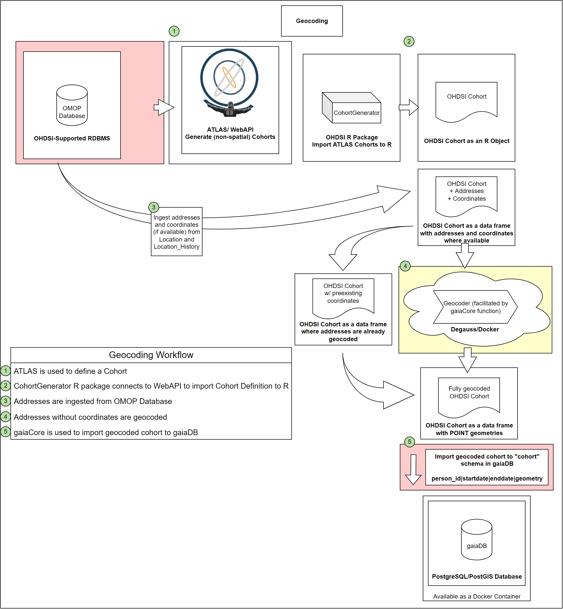
Geocoding Workflow

Overview

This workflow demonstrates how to use the OHDSI Gaia suite of GIS tools to geocode the patient addresses in an OHDSI cohort, enabling further cohort filtering using geospatial data.

Geocoding Workflow (Cohort Definitions) - Click here to download

Prerequisites

This workflow requires the DatabaseConnector, ROhdsiWebApi, and CohortGenerator packages. For this demonstration, we will be using the Eunomia package as the source OMOP database. We will be using the Demo ATLAS instance hosted by OHDSI.

install.packages("DatabaseConnector")
remotes::install_github("OHDSI/ROhdsiWebApi")
remotes::install_github("OHDSI/CohortGenerator")
remotes::install_github("OHDSI/Eunomia")

Configuring Connection to the Servers

We need to configure connections to two servers: the server hosting the OMOP database and the server hosting the gaiaDB Postgres database.

Connect to OMOP server:

library(DatabaseConnector)
connectionDetails <- createConnectionDetails(
  dbms = "postgresql",
  server = "localhost/ohdsi",
  user = "myUser",
  password = "mySecretPassword"
)

For the purposes of this example, we will use the Eunomia test CDM package that is in an Sqlite database stored locally.

connectionDetails <- Eunomia::getEunomiaConnectionDetails()
cdmDatabaseSchema <- "main"
tempEmulationSchema <- NULL
cohortDatabaseSchema <- "main"
cohortTable <- "cohort"

Eunomia does not include location information. We are going to add random US addresses to the Eunomia database for this demonstration.

Start by getting a “fake” address for each person in the Eunomia database:

# TODO add openadds addresses

library(openadds)

# Get all datasets
datasets <- openadds::oa_list()

# Filter datasets to those covering Massachusetts
ma_datasets <- datasets[grep("us/ma/statewide", datasets$source),]

# Download the data for the dataset
data <- oa_get(ma_datasets$processed)[[1]]

data_sample <- data[sample(1:nrow(data), 2694, replace = FALSE), ]

Now we’ll create a location table in Eunomia and assign the location_ids to the records in the person table:

location <- dplyr::mutate(data_sample,
                          LOCATION_ID = 1:nrow(data_sample),
                          ADDRESS_1 = paste(NUMBER, STREET),
                          ADDRESS_2 = UNIT) %>% 
  dplyr::select(
    LOCATION_ID,
    ADDRESS_1,
    ADDRESS_2,
    CITY,
    STATE = REGION,
    ZIP = POSTCODE,
    COUNTY = DISTRICT,
    LOCATION_SOURCE_VALUE = HASH
  )

# Load
conn <- DatabaseConnector::connect(connectionDetails)
DatabaseConnector::dbWriteTable(conn, "location", location, overwrite = TRUE)
# Attach to person records
amendedPersonTable <- DatabaseConnector::querySql(con, 'SELECT * FROM main.person') %>% 
  dplyr::mutate(LOCATION_ID = PERSON_ID)
DatabaseConnector::dbWriteTable(conn, "person", amendedPersonTable, overwrite = TRUE)
DatabaseConnector::disconnect(conn)

Connect to gaiaDB server:

If you don’t already have a gaiaDB server set up, see the installation instructions before proceeding.

library(DatabaseConnector)
gaiaConnectionDetails <- DatabaseConnector::createConnectionDetails(
  dbms = "postgresql",
  server = "localhost/gaiaDB",
  port = 5432,
  user="postgres",
  password = "mySecretPassword") 

Prequisites: Cohort Definition

P1. Define a cohort using ATLAS

Use the OHDSI ATLAS tool to define a cohort. This example uses a cohort definition with an entry event of “Heart Failure” condition occurrence (316139) at age 65 or older. We refer to the WebAPI base URL and the ID of our cohort definition:

baseUrl <- "https://atlas-demo.ohdsi.org/WebAPI"
cohortIds <- c(1782669)

P2. Import the ATLAS Cohort Definition to R

Use the ROhdsiWebApi tool to import the cohort definition to R.

cohortDefinitionSet <- ROhdsiWebApi::exportCohortDefinitionSet(
  baseUrl = baseUrl,
  cohortIds = cohortIds,
  generateStats = TRUE
)

P3. Generate Cohort from the Cohort Definition

Use the CohortGenerator package to create cohort tables in the database cohort schema and generate the cohort set.

cohortTableNames <- CohortGenerator::getCohortTableNames(cohortTable = cohortTable)

# Next create the tables on the database
CohortGenerator::createCohortTables(
  connectionDetails = connectionDetails,
  cohortTableNames = cohortTableNames,
  cohortDatabaseSchema = cohortDatabaseSchema,
  incremental = FALSE
)

# Generate the cohort set
CohortGenerator::generateCohortSet(
  connectionDetails = connectionDetails,
  cdmDatabaseSchema = cdmDatabaseSchema,
  cohortDatabaseSchema = cohortDatabaseSchema,
  cohortTableNames = cohortTableNames,
  cohortDefinitionSet = cohortDefinitionSet,
  incremental = FALSE
)

# Pull the cohort table into R
conn <- DatabaseConnector::connect(connectionDetails)
cohortDataframe <- DatabaseConnector::querySql(con,
                                               'SELECT * FROM main.cohort')
DatabaseConnector::disconnect(conn)

Geocoding

Step 1. Ingest Addresses from OMOP Database

Use the gaiaCore function getCohortAddresses() to extract addresses from OMOP and attach them to our cohort table:

cohortWithAddresses <- getCohortAddresses(connectionDetails = connectionDetails,
                                          cdmDatabaseSchema = cdmDatabaseSchema,
                                          cohort = cohortDataframe)

Step 2. Split cohort dataframe into two tables based on whether it already contains latitude and longitude information

splitResult <- splitAddresses(addressTable = cohortWithAddresses)

alreadyGeocodedCohort <- splitResult$geocoded

notGeocodedCohort <- splitResult$ungeocoded

Step 3. Geocode Addresses without Coordinates

geocodedCohort <- geocodeAddresses(addressTable = notGeocodedCohort)

Step 4. Stack pre-populated and newly geocoded location tables

fullyGeocodedCohort <- geocodedCohort
if (!is.null(alreadyGeocodedCohort)) {
  names(alreadyGeocodedCohort) <- tolower(names(alreadyGeocodedCohort))
  alreadyGeocodedCohort <- dplyr::mutate(alreadyGeocodedCohort, lat = latitude, lon = longitude)
  alreadyGeocodedCohort <- dplyr::select(alreadyGeocodedCohort, names(fullyGeocodedCohort))
  alreadyGeocodedCohort <- sf::st_as_sf(boundGeocodedTable, coords = c("lon", "lat"), crs = 4326)
  fullyGeocodedCohort <- rbind(fullyGeocodedCohort, alreadyGeocodedCohort)
}

Step 5. Import Geocoded Cohort to gaiaDB Database

importCohortTable(gaiaConnectionDetails = gaiaConnectionDetails,
                  cohort = fullyGeocodedCohort)

Step 6. Filter Cohort using PostGIS Functionality

We are going to filter the cohort based on proximity to a temperature sensor. For this example, we only want to include patients whose current address is within about 11.1 km of an EPA air temperature sensor that recorded a temperature greater than 101 degrees Fahrenheit in 2018, 2019, or 2020:

conn <-  DatabaseConnector::connect(gaiaConnectionDetails)

x <- DatabaseConnector::querySql(conn, sql ="select *
    from cohort.cohort_", 1782669, " ct
    where exists (
        select 1
        from (
            select *
    -- This join is ideally made automatically. User should specify a variable (by name)
    -- and threshold (i.e. 101 deg F, 11km radius)
  -- This union is also ideally automatic. In the case of no time constraint, it 
  -- should union all attr_daily_temp_*
            from (
                select * from 
                epa_aqs.attr_daily_temp_2020 a20
                union
                select * from
                epa_aqs.attr_daily_temp_2019 a19
                union
                select * from
                epa_aqs.attr_daily_temp_2018 a18
            )  adt
            inner join epa_aqs.geom_aqs_sites gas 
            on adt.geom_record_id = gas.geom_record_id 
            and variable_source_record_id IN (29, 27, 25)
            and value_as_number > 101
        ) c
        where st_distance(
            ct.geometry,
            c.geom_local_value) < .1 -- degrees, approx 11.1km      
        )")

DatabaseConnector::disconnect(conn)