Summarise observation period
Source:vignettes/articles/summarise_observation_period.Rmd
summarise_observation_period.RmdIntroduction
In this vignette, we will explore the OmopSketch functions
designed to provide an overview of the observation_period
table. Specifically, there are 3 key functions that facilitate this:
-
summariseObservationPeriod(): get some overall statistics describing theobservation_periodtable -
plotObservationPeriod(): create plots showing the results -
tableObservationPeriod(): display the results in a formatted table
Create a mock cdm
Let’s see an example of its functionalities. To start with, we will load essential packages and create a mock cdm using the R package omock.
library(dplyr)
#>
#> Attaching package: 'dplyr'
#> The following objects are masked from 'package:stats':
#>
#>     filter, lag
#> The following objects are masked from 'package:base':
#>
#>     intersect, setdiff, setequal, union
library(OmopSketch)
library(omock)

# Connect to mock database
cdm <- mockCdmFromDataset(datasetName = "GiBleed", source = "duckdb")
#> ℹ Loading bundled GiBleed tables from package data.
#> ℹ Adding drug_strength table.
#> ℹ Creating local <cdm_reference> object.
#> ℹ Inserting <cdm_reference> into duckdb.
Summarise observation periods
Let’s now use the summariseObservationPeriod() function
from the OmopSketch package to generate an overview of
the observation_period table.
This function provides both a general summary of the table and some
detailed statistics, such as the Number of subjects and
the Duration in days for each observation period (e.g.,
first, second, etc.).
summarisedResult <- summariseObservationPeriod(cdm = cdm)

summarisedResult
#> # A tibble: 3,126 × 13
#>    result_id cdm_name group_name            group_level strata_name strata_level
#>        <int> <chr>    <chr>                 <chr>       <chr>       <chr>
#>  1         1 GiBleed  observation_period_o… all         overall     overall
#>  2         1 GiBleed  observation_period_o… all         overall     overall
#>  3         1 GiBleed  observation_period_o… all         overall     overall
#>  4         1 GiBleed  observation_period_o… all         overall     overall
#>  5         1 GiBleed  observation_period_o… all         overall     overall
#>  6         1 GiBleed  observation_period_o… all         overall     overall
#>  7         1 GiBleed  observation_period_o… all         overall     overall
#>  8         1 GiBleed  observation_period_o… all         overall     overall
#>  9         1 GiBleed  observation_period_o… all         overall     overall
#> 10         1 GiBleed  observation_period_o… all         overall     overall
#> # ℹ 3,116 more rows
#> # ℹ 7 more variables: variable_name <chr>, variable_level <chr>,
#> #   estimate_name <chr>, estimate_type <chr>, estimate_value <chr>,
#> #   additional_name <chr>, additional_level <chr>
Notice that the output is in the summarised result format.
We can use the function arguments to specify which summary statistics to compute. For instance, the estimates argument allows us to define which estimates we want to calculate for variables such as the Duration in days of the observation period or the Number of records per person.
summarisedResult <- summariseObservationPeriod(
  cdm = cdm,
  estimates = c("mean", "sd", "q05", "q95")
)

summarisedResult |>
  filter(variable_name == "Duration in days") |>
  select(group_level, variable_name, estimate_name, estimate_value)
#> # A tibble: 8 × 4
#>   group_level variable_name    estimate_name estimate_value
#>   <chr>       <chr>            <chr>         <chr>
#> 1 all         Duration in days mean          14402.0014972862
#> 2 all         Duration in days sd            8725.3408283113
#> 3 all         Duration in days q05           1436
#> 4 all         Duration in days q95           29132.9
#> 5 1st         Duration in days mean          14402.0014972862
#> 6 1st         Duration in days sd            8725.3408283113
#> 7 1st         Duration in days q05           1436
#> 8 1st         Duration in days q95           29132.9
By default, the function returns statistics for the Number of subjects, Duration in days, and Days to next observation both overall and by each ordinal observation period (for example, first, second, etc.).
If we are only interested in overall statistics rather than those
broken down by ordinal period, we can set the argument
byOrdinal = FALSE:
summarisedResult <- summariseObservationPeriod(
  cdm = cdm,
  estimates = c("mean", "sd", "q05", "q95"),
  byOrdinal = FALSE
)

summarisedResult |>
  filter(variable_name == "Duration in days") |>
  distinct(group_name, group_level)
#> # A tibble: 1 × 2
#>   group_name                 group_level
#>   <chr>                      <chr>
#> 1 observation_period_ordinal all
Missingness
When the argument missingData = TRUE is set, the results
will include an overall summary of missing data in the table, including
the number of 0s in the concept columns. This output is
analogous to the results produced by the OmopSketch function
summariseMissingData().
summarisedResult <- summariseObservationPeriod(
  cdm = cdm,
  estimates = c("mean", "sd", "q05", "q95"),
  missingData = TRUE
)

summarisedResult |>
  filter(variable_name == "Column name") |>
  select(group_level, variable_name, estimate_name, estimate_value)
#> # A tibble: 16 × 4
#>    group_level variable_name estimate_name   estimate_value
#>    <chr>       <chr>         <chr>           <chr>
#>  1 all         Column name   na_count        0
#>  2 all         Column name   na_percentage   0.00
#>  3 all         Column name   zero_count      0
#>  4 all         Column name   zero_percentage 0.00
#>  5 all         Column name   na_count        0
#>  6 all         Column name   na_percentage   0.00
#>  7 all         Column name   zero_count      0
#>  8 all         Column name   zero_percentage 0.00
#>  9 all         Column name   na_count        0
#> 10 all         Column name   na_percentage   0.00
#> 11 all         Column name   na_count        0
#> 12 all         Column name   na_percentage   0.00
#> 13 all         Column name   na_count        0
#> 14 all         Column name   na_percentage   0.00
#> 15 all         Column name   zero_count      0
#> 16 all         Column name   zero_percentage 0.00
Quality
When the argument quality = TRUE is set, the results
will include a quality assessment of the observation period table.
This assessment provides information such as:
- Issues with date columns (e.g., start dates occurring after end
dates, or dates preceding a subject’s birth date).
- The presence of
person_idvalues that do not exist in thepersontable. - A summary of the types of concept_id available in the table.
summarisedResult <- summariseObservationPeriod(
  cdm = cdm,
  estimates = "mean",
  missingData = FALSE,
  quality = TRUE
)

summarisedResult |>
  select(group_level, variable_name, variable_level, estimate_name, estimate_value)
#> # A tibble: 14 × 5
#>    group_level variable_name         variable_level estimate_name estimate_value
#>    <chr>       <chr>                 <chr>          <chr>         <chr>
#>  1 all         Records per person    NA             mean          1
#>  2 all         Duration in days      NA             mean          14402.0014972…
#>  3 1st         Duration in days      NA             mean          14402.0014972…
#>  4 all         Number records        NA             count         5343
#>  5 all         Number subjects       NA             count         5343
#>  6 1st         Number subjects       NA             count         5343
#>  7 all         Type concept id       Period coveri… count         5343
#>  8 all         Subjects not in pers… NA             count         2649
#>  9 all         Subjects not in pers… NA             percentage    49.58
#> 10 all         End date before star… NA             count         0
#> 11 all         Start date before bi… NA             count         0
#> 12 all         Type concept id       Period coveri… percentage    100.00
#> 13 all         End date before star… NA             percentage    0.00
#> 14 all         Start date before bi… NA             percentage    0.00
Strata
It is also possible to stratify the results by sex and age groups:
summarisedResult <- summariseObservationPeriod(
  cdm = cdm,
  estimates = c("mean", "sd", "q05", "q95"),
  sex = TRUE,
  ageGroup = list("<35" = c(0, 34), ">=35" = c(35, Inf)),
)
Notice that, by default, the “overall” group will be also included,
as well as crossed strata (that means, sex == "Female" and
ageGroup == "\>35").
Tidy the summarised object
tableObservationPeriod() will help you to create a table
(see supported types with: visOmopResults::tableType()). By
default it creates a gt table.
summarisedResult <- summariseObservationPeriod(
  cdm = cdm,
  estimates = c("mean", "sd", "q05", "q95"),
  sex = TRUE
)

summarisedResult |>
tableObservationPeriod(type = "gt")| Observation period ordinal | Variable name | Variable level | Is required | Estimate name |
Data source
|
|---|---|---|---|---|---|
| GiBleed | |||||
| overall | |||||
| all | Number records | – | overall | N | 5,343 |
| Number subjects | – | overall | N | 5,343 | |
| Subjects not in person table | – | overall | N (%) | 2,649 (49.58%) | |
| Records per person | – | overall | Mean (SD) | 1.00 (0.00) | |
| Duration in days | – | overall | Mean (SD) | 14,402.00 (8,725.34) | |
| Type concept id | Period covering healthcare encounters | overall | N (%) | 5,343 (100.00%) | |
| Start date before birth date | – | overall | N (%) | 0 (0.00%) | |
| End date before start date | – | overall | N (%) | 0 (0.00%) | |
| Column name | Observation period end date | TRUE | N missing data (%) | 0 (0.00%) | |
| Observation period id | TRUE | N missing data (%) | 0 (0.00%) | ||
| N zeros (%) | 0 (0.00%) | ||||
| Observation period start date | TRUE | N missing data (%) | 0 (0.00%) | ||
| Period type concept id | TRUE | N missing data (%) | 0 (0.00%) | ||
| N zeros (%) | 0 (0.00%) | ||||
| Person id | TRUE | N missing data (%) | 0 (0.00%) | ||
| N zeros (%) | 0 (0.00%) | ||||
| 1st | Number subjects | – | overall | N | 5,343 |
| Duration in days | – | overall | Mean (SD) | 14,402.00 (8,725.34) | |
| Female | |||||
| all | Number records | – | overall | N | 1,373 |
| Number subjects | – | overall | N | 1,373 | |
| Records per person | – | overall | Mean (SD) | 1.00 (0.00) | |
| Duration in days | – | overall | Mean (SD) | 21,666.77 (5,623.53) | |
| Type concept id | Period covering healthcare encounters | overall | N (%) | 1,373 (100.00%) | |
| Column name | Observation period end date | TRUE | N missing data (%) | 0 (0.00%) | |
| Observation period id | TRUE | N missing data (%) | 0 (0.00%) | ||
| N zeros (%) | 0 (0.00%) | ||||
| Observation period start date | TRUE | N missing data (%) | 0 (0.00%) | ||
| Period type concept id | TRUE | N missing data (%) | 0 (0.00%) | ||
| N zeros (%) | 0 (0.00%) | ||||
| Person id | TRUE | N missing data (%) | 0 (0.00%) | ||
| N zeros (%) | 0 (0.00%) | ||||
| 1st | Number subjects | – | overall | N | 1,373 |
| Duration in days | – | overall | Mean (SD) | 21,666.77 (5,623.53) | |
| Male | |||||
| all | Number records | – | overall | N | 1,321 |
| Number subjects | – | overall | N | 1,321 | |
| Records per person | – | overall | Mean (SD) | 1.00 (0.00) | |
| Duration in days | – | overall | Mean (SD) | 21,535.91 (5,287.44) | |
| Type concept id | Period covering healthcare encounters | overall | N (%) | 1,321 (100.00%) | |
| Column name | Observation period end date | TRUE | N missing data (%) | 0 (0.00%) | |
| Observation period id | TRUE | N missing data (%) | 0 (0.00%) | ||
| N zeros (%) | 0 (0.00%) | ||||
| Observation period start date | TRUE | N missing data (%) | 0 (0.00%) | ||
| Period type concept id | TRUE | N missing data (%) | 0 (0.00%) | ||
| N zeros (%) | 0 (0.00%) | ||||
| Person id | TRUE | N missing data (%) | 0 (0.00%) | ||
| N zeros (%) | 0 (0.00%) | ||||
| 1st | Number subjects | – | overall | N | 1,321 |
| Duration in days | – | overall | Mean (SD) | 21,535.91 (5,287.44) | |
| None | |||||
| all | Number records | – | overall | N | 2,649 |
| Number subjects | – | overall | N | 2,649 | |
| Records per person | – | overall | Mean (SD) | 1.00 (0.00) | |
| Duration in days | – | overall | Mean (SD) | 7,079.08 (4,106.70) | |
| Type concept id | Period covering healthcare encounters | overall | N (%) | 2,649 (100.00%) | |
| Column name | Observation period end date | TRUE | N missing data (%) | 0 (0.00%) | |
| Observation period id | TRUE | N missing data (%) | 0 (0.00%) | ||
| N zeros (%) | 0 (0.00%) | ||||
| Observation period start date | TRUE | N missing data (%) | 0 (0.00%) | ||
| Period type concept id | TRUE | N missing data (%) | 0 (0.00%) | ||
| N zeros (%) | 0 (0.00%) | ||||
| Person id | TRUE | N missing data (%) | 0 (0.00%) | ||
| N zeros (%) | 0 (0.00%) | ||||
| 1st | Number subjects | – | overall | N | 2,649 |
| Duration in days | – | overall | Mean (SD) | 7,079.08 (4,106.70) | |
Visualise the results
Finally, we can visualise the result using
plotObservationPeriod().
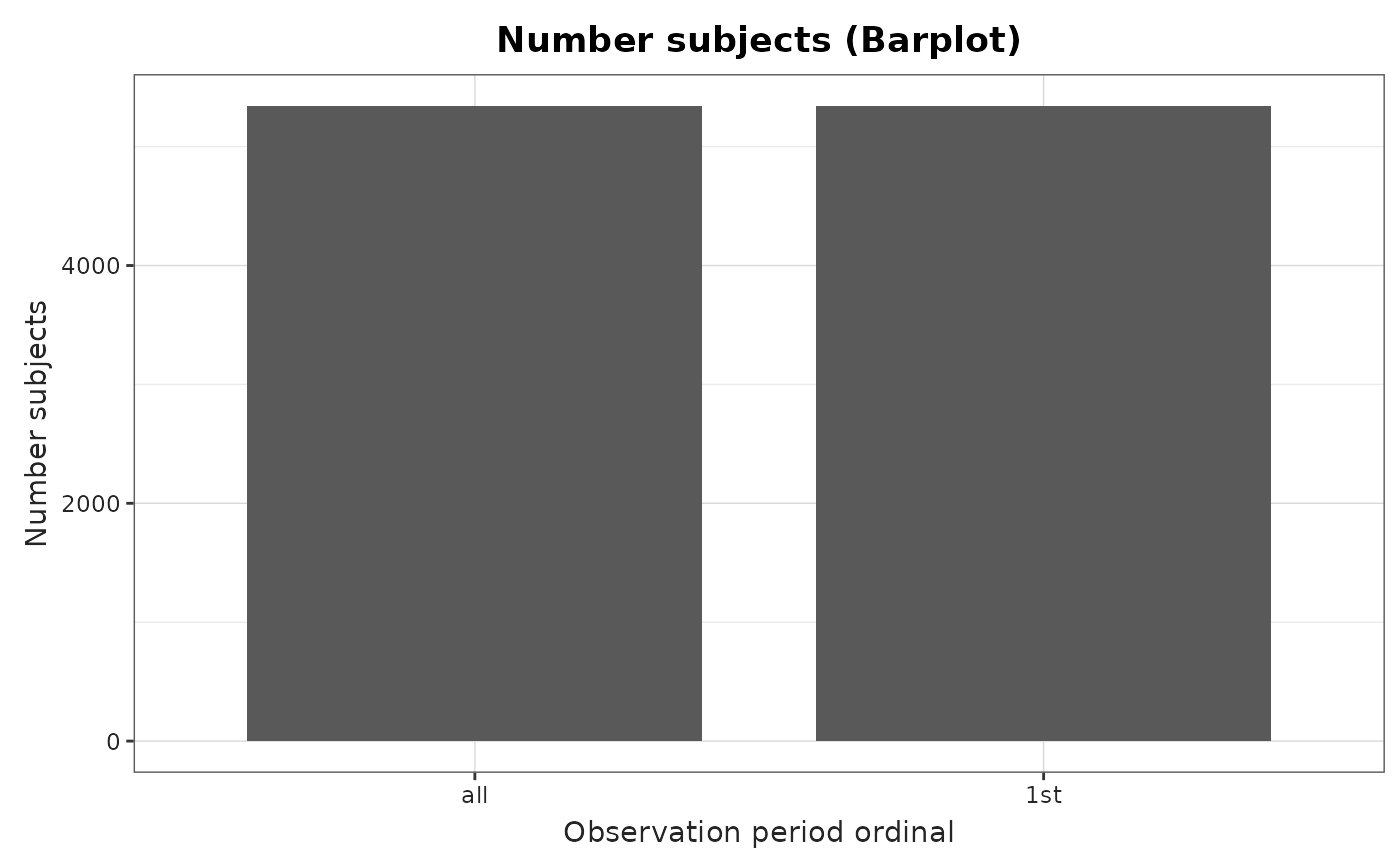
summarisedResult <- summariseObservationPeriod(cdm = cdm)

plotObservationPeriod(
  result = summarisedResult,
  variableName = "Number subjects",
  plotType = "barplot"
)
Note that either Number subjects or
Duration in days can be plotted. For
Number of subjects, the plot type can be
barplot, whereas for Duration in days, the
plot type can be barplot, boxplot, or
densityplot.”
Additionally, if results were stratified by sex or age group, we can
further use facet or colour arguments to
highlight the different results in the plot. To help us identify by
which variables we can colour or facet by, we can use visOmopResult
package.
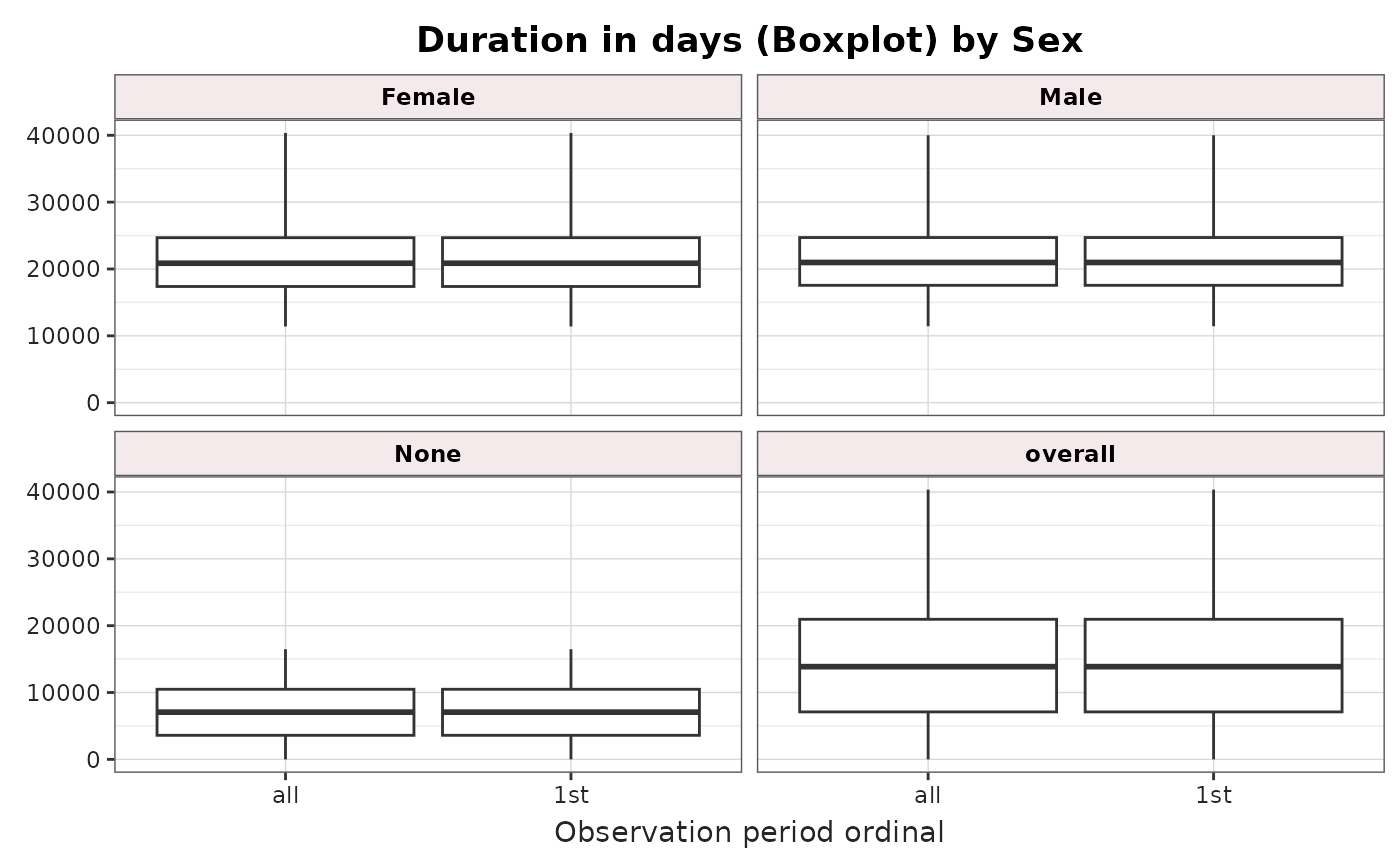
summarisedResult <- summariseObservationPeriod(cdm = cdm, sex = TRUE)

plotObservationPeriod(
  result = summarisedResult,
  variableName = "Duration in days",
  plotType = "boxplot",
  facet = "sex"
)
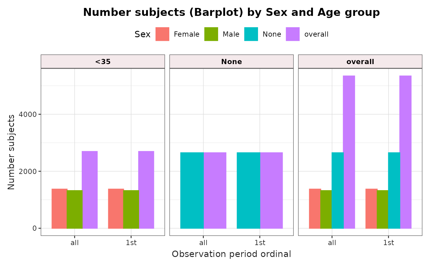
summarisedResult <- summariseObservationPeriod(
  cdm = cdm,
  sex = TRUE,
  ageGroup = list("<35" = c(0, 34), ">=35" = c(35, Inf))
)

plotObservationPeriod(
  result = summarisedResult,
  colour = "sex",
  facet = "age_group"
)