Summarise temporal trends in OMOP tables • OmopSketch

Introduction

In this vignette, we will explore the OmopSketch function summariseTrend(), which summarises temporal trends from OMOP CDM tables. This function allows you to visualise how key measures (such as number of records, number of persons, person-days, age, or sex distribution) change over time.

Create a mock cdm

Let’s start by loading essential packages and creating a mock CDM using the R package omock.

library(omock)
library(OmopSketch)
library(dplyr)
#> 
#> Attaching package: 'dplyr'
#> The following objects are masked from 'package:stats':
#> 
#>     filter, lag
#> The following objects are masked from 'package:base':
#> 
#>     intersect, setdiff, setequal, union
library(visOmopResults)

cdm <- mockCdmFromDataset(datasetName = "GiBleed", source = "duckdb")
#> ℹ Loading bundled GiBleed tables from package data.
#> ℹ Adding drug_strength table.
#> ℹ Creating local <cdm_reference> object.
#> ℹ Inserting <cdm_reference> into duckdb.

cdm
#> 
#> ── # OMOP CDM reference (duckdb) of GiBleed ────────────────────────────────────
#> • omop tables: care_site, cdm_source, concept, concept_ancestor, concept_class,
#> concept_relationship, concept_synonym, condition_era, condition_occurrence,
#> cost, death, device_exposure, domain, dose_era, drug_era, drug_exposure,
#> drug_strength, fact_relationship, location, measurement, metadata, note,
#> note_nlp, observation, observation_period, payer_plan_period, person,
#> procedure_occurrence, provider, relationship, source_to_concept_map, specimen,
#> visit_detail, visit_occurrence, vocabulary
#> • cohort tables: -
#> • achilles tables: -
#> • other tables: -

Summarise temporal trends

Let’s use summariseTrend() to get an overview of table content over time. In this example, we summarise yearly trends for the event tables condition_occurrence and drug_exposure, and include observation_period as an episode table.

summarisedResult <- summariseTrend(
  cdm = cdm,
  event = c("condition_occurrence", "drug_exposure"),
  episode = "observation_period",
  interval = "years"
)

summarisedResult |>
  glimpse()
#> Rows: 900
#> Columns: 13
#> $ result_id        <int> 1, 1, 2, 2, 2, 2, 1, 1, 1, 1, 2, 2, 2, 2, 1, 1, 1, 1,…
#> $ cdm_name         <chr> "GiBleed", "GiBleed", "GiBleed", "GiBleed", "GiBleed"…
#> $ group_name       <chr> "omop_table", "omop_table", "omop_table", "omop_table…
#> $ group_level      <chr> "condition_occurrence", "condition_occurrence", "obse…
#> $ strata_name      <chr> "overall", "overall", "overall", "overall", "overall"…
#> $ strata_level     <chr> "overall", "overall", "overall", "overall", "overall"…
#> $ variable_name    <chr> "Number of records", "Number of records", "Number of …
#> $ variable_level   <chr> NA, NA, NA, NA, NA, NA, NA, NA, NA, NA, NA, NA, NA, N…
#> $ estimate_name    <chr> "count", "percentage", "count", "count", "percentage"…
#> $ estimate_type    <chr> "integer", "percentage", "integer", "integer", "perce…
#> $ estimate_value   <chr> "1", "0.00", "2", "0", "0.04", "0.00", "4", "0.01", "…
#> $ additional_name  <chr> "time_interval", "time_interval", "time_interval", "t…
#> $ additional_level <chr> "1908-01-01 to 1908-12-31", "1908-01-01 to 1908-12-31…

Notice that the output is in the summarised result format.

What are event and episode tables?

Event tables capture records that are assigned to a single point in time for trend summaries (for example, a diagnosis, drug exposure start, or measurement). Event records are included when their start date falls within the study period, and each record contributes to the interval containing its start date.
Episode tables describe periods that span time (for example, observation periods or eras). Episode records are included when their start or end date overlaps the study period. They are trimmed to the study period and can contribute to every interval they overlap.

You can check whether a table was treated as an event or an episode table in the settings of the summarised result:

summarisedResult |>
  addSettings(settingsColumn = "type") |>
  glimpse()
#> Rows: 900
#> Columns: 14
#> $ result_id        <int> 1, 1, 2, 2, 2, 2, 1, 1, 1, 1, 2, 2, 2, 2, 1, 1, 1, 1,…
#> $ cdm_name         <chr> "GiBleed", "GiBleed", "GiBleed", "GiBleed", "GiBleed"…
#> $ group_name       <chr> "omop_table", "omop_table", "omop_table", "omop_table…
#> $ group_level      <chr> "condition_occurrence", "condition_occurrence", "obse…
#> $ strata_name      <chr> "overall", "overall", "overall", "overall", "overall"…
#> $ strata_level     <chr> "overall", "overall", "overall", "overall", "overall"…
#> $ variable_name    <chr> "Number of records", "Number of records", "Number of …
#> $ variable_level   <chr> NA, NA, NA, NA, NA, NA, NA, NA, NA, NA, NA, NA, NA, N…
#> $ estimate_name    <chr> "count", "percentage", "count", "count", "percentage"…
#> $ estimate_type    <chr> "integer", "percentage", "integer", "integer", "perce…
#> $ estimate_value   <chr> "1", "0.00", "2", "0", "0.04", "0.00", "4", "0.01", "…
#> $ additional_name  <chr> "time_interval", "time_interval", "time_interval", "t…
#> $ additional_level <chr> "1908-01-01 to 1908-12-31", "1908-01-01 to 1908-12-31…
#> $ type             <chr> "event", "event", "episode", "episode", "episode", "e…

Outputs

You can choose what to summarise using the output argument. Options include:

"record": number of records (default value).
"person": number of distinct subjects.
"person-days": number of person-days (episode tables only).
"age": median age.
"sex": number of females.

Records

For each time interval, the results include the number of records during that period. In addition to absolute counts, the function reports the percentage of records in each interval relative to the total number of records in the table after any date restriction.

summarisedResult <- summariseTrend(
  cdm = cdm,
  event = "condition_occurrence",
  output = "record",
  interval = "years"
)

summarisedResult |>
  select(group_level, variable_name, additional_level, estimate_name, estimate_value)
#> # A tibble: 226 × 5
#>    group_level       variable_name additional_level estimate_name estimate_value
#>    <chr>             <chr>         <chr>            <chr>         <chr>         
#>  1 condition_occurr… Number of re… 1908-01-01 to 1… count         1             
#>  2 condition_occurr… Number of re… 1908-01-01 to 1… percentage    0.00          
#>  3 condition_occurr… Number of re… 1909-01-01 to 1… count         4             
#>  4 condition_occurr… Number of re… 1909-01-01 to 1… percentage    0.01          
#>  5 condition_occurr… Number of re… 1910-01-01 to 1… count         16            
#>  6 condition_occurr… Number of re… 1910-01-01 to 1… percentage    0.02          
#>  7 condition_occurr… Number of re… 1911-01-01 to 1… count         18            
#>  8 condition_occurr… Number of re… 1911-01-01 to 1… percentage    0.03          
#>  9 condition_occurr… Number of re… 1912-01-01 to 1… count         31            
#> 10 condition_occurr… Number of re… 1912-01-01 to 1… percentage    0.05          
#> # ℹ 216 more rows

For episode tables with output = "record" and a time interval such as "years", record counts are split into two measures: Number of records: start_date counts episodes that start in each interval, and Number of records: end_date counts episodes that end in each interval. The overall result still uses Number of records for the total number of episode records.

For example, using observation_period as an episode table:

summarisedResult <- summariseTrend(
  cdm = cdm,
  episode = "observation_period",
  output = "record",
  interval = "years"
)

summarisedResult |>
  filter(grepl("Number of records", variable_name)) |>
  select(variable_name, additional_level, estimate_name, estimate_value)
#> # A tibble: 450 × 4
#>    variable_name                 additional_level   estimate_name estimate_value
#>    <chr>                         <chr>              <chr>         <chr>         
#>  1 Number of records: start_date 1908-01-01 to 190… count         2             
#>  2 Number of records: end_date   1908-01-01 to 190… count         0             
#>  3 Number of records: start_date 1908-01-01 to 190… percentage    0.04          
#>  4 Number of records: end_date   1908-01-01 to 190… percentage    0.00          
#>  5 Number of records: start_date 1909-01-01 to 190… count         22            
#>  6 Number of records: end_date   1909-01-01 to 190… count         0             
#>  7 Number of records: start_date 1909-01-01 to 190… percentage    0.41          
#>  8 Number of records: end_date   1909-01-01 to 190… percentage    0.00          
#>  9 Number of records: start_date 1910-01-01 to 191… count         28            
#> 10 Number of records: end_date   1910-01-01 to 191… count         0             
#> # ℹ 440 more rows

Subjects

For each time interval, output = "person" returns the number of distinct subjects with records during that period. The percentage estimate uses the number of subjects in the person table as the denominator.

summarisedResult <- summariseTrend(
  cdm = cdm,
  event = "condition_occurrence",
  output = "person",
  interval = "years"
)

summarisedResult |>
  select(group_level, variable_name, additional_level, estimate_name, estimate_value)
#> # A tibble: 226 × 5
#>    group_level       variable_name additional_level estimate_name estimate_value
#>    <chr>             <chr>         <chr>            <chr>         <chr>         
#>  1 condition_occurr… Number of su… 1908-01-01 to 1… count         1             
#>  2 condition_occurr… Number of su… 1908-01-01 to 1… percentage    0.04          
#>  3 condition_occurr… Number of su… 1909-01-01 to 1… count         4             
#>  4 condition_occurr… Number of su… 1909-01-01 to 1… percentage    0.15          
#>  5 condition_occurr… Number of su… 1910-01-01 to 1… count         13            
#>  6 condition_occurr… Number of su… 1910-01-01 to 1… percentage    0.48          
#>  7 condition_occurr… Number of su… 1911-01-01 to 1… count         13            
#>  8 condition_occurr… Number of su… 1911-01-01 to 1… percentage    0.48          
#>  9 condition_occurr… Number of su… 1912-01-01 to 1… count         21            
#> 10 condition_occurr… Number of su… 1912-01-01 to 1… percentage    0.78          
#> # ℹ 216 more rows

Person-days

When an episode table is specified, you can include "person-days" in the output to summarise total follow-up time across intervals. The results include both the number of person-days in each interval and the percentage relative to the total person-days in the episode table after any date restriction.

summarisedResult <- summariseTrend(
  cdm = cdm,
  episode = "observation_period",
  output = "person-days",
  interval = "years"
)

summarisedResult |>
  select(group_level, variable_name, additional_level, estimate_name, estimate_value)
#> # A tibble: 226 × 5
#>    group_level       variable_name additional_level estimate_name estimate_value
#>    <chr>             <chr>         <chr>            <chr>         <chr>         
#>  1 observation_peri… Person-days   1908-01-01 to 1… count         175           
#>  2 observation_peri… Person-days   1908-01-01 to 1… percentage    0.00          
#>  3 observation_peri… Person-days   1909-01-01 to 1… count         4636          
#>  4 observation_peri… Person-days   1909-01-01 to 1… percentage    0.01          
#>  5 observation_peri… Person-days   1910-01-01 to 1… count         9946          
#>  6 observation_peri… Person-days   1910-01-01 to 1… percentage    0.01          
#>  7 observation_peri… Person-days   1911-01-01 to 1… count         13031         
#>  8 observation_peri… Person-days   1911-01-01 to 1… percentage    0.02          
#>  9 observation_peri… Person-days   1912-01-01 to 1… count         16986         
#> 10 observation_peri… Person-days   1912-01-01 to 1… percentage    0.02          
#> # ℹ 216 more rows

The function automatically skips "person-days" for event tables.

summarisedResult <- summariseTrend(
  cdm = cdm,
  event = "visit_occurrence",
  output = "person-days",
  interval = "years"
)
#> → The number of person-days is not computed for event tables
summarisedResult
#> # A tibble: 0 × 13
#> # ℹ 13 variables: result_id <int>, cdm_name <chr>, group_name <chr>,
#> #   group_level <chr>, strata_name <chr>, strata_level <chr>,
#> #   variable_name <chr>, variable_level <chr>, estimate_name <chr>,
#> #   estimate_type <chr>, estimate_value <chr>, additional_name <chr>,
#> #   additional_level <chr>

Age

When "age" is included in the output argument, the function reports the median age of subjects. For event tables, age is calculated at the record start date. For episode tables summarised by interval, age is calculated at the later of the episode start date and the interval start date.

summarisedResult <- summariseTrend(
  cdm = cdm,
  event = "condition_occurrence",
  output = "age",
  interval = "years"
)
#> ℹ The following estimates will be calculated:
#> • age: median
#> → Start summary of data, at 2026-06-17 10:04:47.070199
#> 
#> ✔ Summary finished, at 2026-06-17 10:04:47.765744

summarisedResult |>
  select(variable_name, additional_level, estimate_name, estimate_value)
#> # A tibble: 113 × 4
#>    variable_name additional_level         estimate_name estimate_value
#>    <chr>         <chr>                    <chr>         <chr>         
#>  1 Age           1908-01-01 to 1908-12-31 median        0             
#>  2 Age           1909-01-01 to 1909-12-31 median        0             
#>  3 Age           1910-01-01 to 1910-12-31 median        1             
#>  4 Age           1911-01-01 to 1911-12-31 median        1             
#>  5 Age           1912-01-01 to 1912-12-31 median        1             
#>  6 Age           1913-01-01 to 1913-12-31 median        2             
#>  7 Age           1914-01-01 to 1914-12-31 median        3             
#>  8 Age           1915-01-01 to 1915-12-31 median        3             
#>  9 Age           1916-01-01 to 1916-12-31 median        4             
#> 10 Age           1917-01-01 to 1917-12-31 median        5             
#> # ℹ 103 more rows

Sex

When "sex" is included in the output argument, the function counts the number of female subjects in each time interval. It also provides the percentage of females relative to subjects with a recorded male or female sex in the table after any date restriction.

summarisedResult <- summariseTrend(
  cdm = cdm,
  event = "condition_occurrence",
  output = "sex",
  interval = "years"
)
summarisedResult |>
  select(variable_name, additional_level, estimate_name, estimate_value)
#> # A tibble: 226 × 4
#>    variable_name     additional_level         estimate_name estimate_value
#>    <chr>             <chr>                    <chr>         <chr>         
#>  1 Number of females 1908-01-01 to 1908-12-31 count         1             
#>  2 Number of females 1908-01-01 to 1908-12-31 percentage    0.04          
#>  3 Number of females 1909-01-01 to 1909-12-31 count         4             
#>  4 Number of females 1909-01-01 to 1909-12-31 percentage    0.15          
#>  5 Number of females 1910-01-01 to 1910-12-31 count         12            
#>  6 Number of females 1910-01-01 to 1910-12-31 percentage    0.45          
#>  7 Number of females 1911-01-01 to 1911-12-31 count         9             
#>  8 Number of females 1911-01-01 to 1911-12-31 percentage    0.33          
#>  9 Number of females 1912-01-01 to 1912-12-31 count         16            
#> 10 Number of females 1912-01-01 to 1912-12-31 percentage    0.59          
#> # ℹ 216 more rows

Intervals

The interval argument controls the temporal granularity of the results. Possible values are "overall" (default, no stratification by time), "years", "quarters", and "months".

For example, to see quarterly trends:

summarisedResult <- summariseTrend(
  cdm = cdm,
  event = "condition_occurrence",
  interval = "quarters",
  output = "record"
)

summarisedResult |>
  select(additional_level, estimate_value)
#> # A tibble: 884 × 2
#>    additional_level         estimate_value
#>    <chr>                    <chr>         
#>  1 1908-10-01 to 1908-12-31 1             
#>  2 1908-10-01 to 1908-12-31 0.00          
#>  3 1909-04-01 to 1909-06-30 2             
#>  4 1909-04-01 to 1909-06-30 0.00          
#>  5 1909-07-01 to 1909-09-30 2             
#>  6 1909-07-01 to 1909-09-30 0.00          
#>  7 1910-01-01 to 1910-03-31 4             
#>  8 1910-01-01 to 1910-03-31 0.01          
#>  9 1910-04-01 to 1910-06-30 4             
#> 10 1910-04-01 to 1910-06-30 0.01          
#> # ℹ 874 more rows

Stratify by age and sex

You can use the ageGroup and sex arguments to stratify the results. Age groups are assigned using the record start date for event tables and the relevant episode start date or interval start date for episode tables.

summarisedResult <- summariseTrend(
  cdm = cdm,
  event = "condition_occurrence",
  interval = "years",
  output = c("record", "age", "sex"),
  ageGroup = list("<35" = c(0, 34), ">=35" = c(35, Inf)),
  sex = TRUE
)
#> ℹ The following estimates will be calculated:
#> • age: median
#> → Start summary of data, at 2026-06-17 10:04:51.54565
#> 
#> ■■■■■■■■■■■■                    3/8 group-strata combinations @ 2026-06-17 10:0…
#> 
#> ■■■■■■■■■■■■■■■■                4/8 group-strata combinations @ 2026-06-17 10:0…
#> 
#> ■■■■■■■■■■■■■■■■■■■■■■■■■■■■■■■ 8/8 group-strata combinations @ 2026-06-17 10:0…
#> 
#> ✔ Summary finished, at 2026-06-17 10:04:55.048776

summarisedResult |>
  select(variable_name, strata_level, estimate_name, estimate_value)
#> # A tibble: 3,318 × 4
#>    variable_name     strata_level   estimate_name estimate_value
#>    <chr>             <chr>          <chr>         <chr>         
#>  1 Number of records overall        count         1             
#>  2 Number of records <35            count         1             
#>  3 Number of records Female         count         1             
#>  4 Number of records Female &&& <35 count         1             
#>  5 Number of females overall        count         1             
#>  6 Number of females <35            count         1             
#>  7 Age               overall        median        0             
#>  8 Age               <35            median        0             
#>  9 Age               Female         median        0             
#> 10 Age               Female &&& <35 median        0             
#> # ℹ 3,308 more rows

By default, the output includes the “overall” group as well as combined strata (for example, Female and >=35). For output = "sex", sex stratification is not applied because a single estimate summarising the female population is returned.

In-observation stratification

When inObservation = TRUE, the results are stratified by whether each record occurred within the subject’s observation period. For episode records, both the start and end date must fall within an observation period to be labelled as in observation. This can be useful for identifying data quality issues or assessing completeness.

summarisedResult <- summariseTrend(
  cdm = cdm,
  event = "condition_occurrence",
  interval = "overall",
  output = "record",
  inObservation = TRUE
)

summarisedResult |>
  select(variable_name, strata_name, strata_level, estimate_name, estimate_value)
#> # A tibble: 6 × 5
#>   variable_name     strata_name    strata_level estimate_name estimate_value
#>   <chr>             <chr>          <chr>        <chr>         <chr>         
#> 1 Number of records overall        overall      count         65332         
#> 2 Number of records in_observation FALSE        count         85            
#> 3 Number of records in_observation TRUE         count         65247         
#> 4 Number of records overall        overall      percentage    100.00        
#> 5 Number of records in_observation FALSE        percentage    0.13          
#> 6 Number of records in_observation TRUE         percentage    99.87

Date Range

You can restrict the study period using the dateRange argument. Event records are kept when their start date is within the date range. Episode records are kept when they overlap the date range and are trimmed to the requested period.

summarisedResult <- summariseTrend(
  cdm = cdm,
  event = "drug_exposure",
  dateRange = as.Date(c("1990-01-01", "2010-01-01"))
)

summarisedResult |>
  settings() |>
  glimpse()
#> Rows: 1
#> Columns: 12
#> $ result_id          <int> 1
#> $ result_type        <chr> "summarise_trend"
#> $ package_name       <chr> "OmopSketch"
#> $ package_version    <chr> "1.1.0"
#> $ group              <chr> "omop_table"
#> $ strata             <chr> ""
#> $ additional         <chr> ""
#> $ min_cell_count     <chr> "0"
#> $ interval           <chr> "overall"
#> $ study_period_end   <chr> "2010-01-01"
#> $ study_period_start <chr> "1990-01-01"
#> $ type               <chr> "event"

Tidy the summarised object with tableTrend

tableTrend() helps you convert a summarised result into a formatted table for reporting or inspection. The table type can be set with the type argument; supported formats are provided by visOmopResults::tableType(). If type = NULL, global table options are used when available; otherwise, a gt table is created by default.

result <- summariseTrend(
  cdm = cdm,
  event = "condition_occurrence",
  episode = "observation_period",
  output = "age",
  interval = "years"
)
#> ℹ The following estimates will be calculated:
#> • age: median
#> → Start summary of data, at 2026-06-17 10:04:57.248103
#> 
#> ✔ Summary finished, at 2026-06-17 10:04:57.923602
#> ℹ The following estimates will be calculated:
#> • age: median
#> → Start summary of data, at 2026-06-17 10:04:58.654033
#> 
#> ✔ Summary finished, at 2026-06-17 10:04:58.870692
#> ℹ The following estimates will be calculated:
#> • age: median
#> → Start summary of data, at 2026-06-17 10:05:04.192806
#> 
#> ✔ Summary finished, at 2026-06-17 10:05:04.65711
tableTrend(result = result)

Summary of Age by years in condition_occurrence, observation_period tables
Variable name	Time interval	Estimate name	Interval	Database name
Variable name	Time interval	Estimate name	Interval	GiBleed
event; condition_occurrence
Age	1908-01-01 to 1908-12-31	Median	years	0
	1909-01-01 to 1909-12-31	Median	years	0
	1910-01-01 to 1910-12-31	Median	years	1
	1911-01-01 to 1911-12-31	Median	years	1
	1912-01-01 to 1912-12-31	Median	years	1
	1913-01-01 to 1913-12-31	Median	years	2
	1914-01-01 to 1914-12-31	Median	years	3
	1915-01-01 to 1915-12-31	Median	years	3
	1916-01-01 to 1916-12-31	Median	years	4
	1917-01-01 to 1917-12-31	Median	years	5
	1918-01-01 to 1918-12-31	Median	years	6
	1919-01-01 to 1919-12-31	Median	years	6
	1920-01-01 to 1920-12-31	Median	years	6
	1921-01-01 to 1921-12-31	Median	years	4
	1922-01-01 to 1922-12-31	Median	years	4
	1923-01-01 to 1923-12-31	Median	years	5
	1924-01-01 to 1924-12-31	Median	years	4
	1925-01-01 to 1925-12-31	Median	years	5
	1926-01-01 to 1926-12-31	Median	years	6
	1927-01-01 to 1927-12-31	Median	years	7
	1928-01-01 to 1928-12-31	Median	years	8
	1929-01-01 to 1929-12-31	Median	years	9
	1930-01-01 to 1930-12-31	Median	years	9
	1931-01-01 to 1931-12-31	Median	years	9
	1932-01-01 to 1932-12-31	Median	years	11
	1933-01-01 to 1933-12-31	Median	years	11
	1934-01-01 to 1934-12-31	Median	years	13
	1935-01-01 to 1935-12-31	Median	years	12
	1936-01-01 to 1936-12-31	Median	years	12
	1937-01-01 to 1937-12-31	Median	years	7
	1938-01-01 to 1938-12-31	Median	years	11
	1939-01-01 to 1939-12-31	Median	years	6
	1940-01-01 to 1940-12-31	Median	years	5
	1941-01-01 to 1941-12-31	Median	years	5
	1942-01-01 to 1942-12-31	Median	years	7
	1943-01-01 to 1943-12-31	Median	years	7
	1944-01-01 to 1944-12-31	Median	years	8
	1945-01-01 to 1945-12-31	Median	years	7
	1946-01-01 to 1946-12-31	Median	years	8
	1947-01-01 to 1947-12-31	Median	years	8
	1948-01-01 to 1948-12-31	Median	years	9
	1949-01-01 to 1949-12-31	Median	years	8
	1950-01-01 to 1950-12-31	Median	years	6
	1951-01-01 to 1951-12-31	Median	years	6
	1952-01-01 to 1952-12-31	Median	years	6
	1953-01-01 to 1953-12-31	Median	years	7
	1954-01-01 to 1954-12-31	Median	years	7
	1955-01-01 to 1955-12-31	Median	years	8
	1956-01-01 to 1956-12-31	Median	years	7
	1957-01-01 to 1957-12-31	Median	years	9
	1958-01-01 to 1958-12-31	Median	years	7
	1959-01-01 to 1959-12-31	Median	years	8
	1960-01-01 to 1960-12-31	Median	years	8
	1961-01-01 to 1961-12-31	Median	years	8
	1962-01-01 to 1962-12-31	Median	years	8
	1963-01-01 to 1963-12-31	Median	years	9
	1964-01-01 to 1964-12-31	Median	years	9
	1965-01-01 to 1965-12-31	Median	years	9
	1966-01-01 to 1966-12-31	Median	years	10
	1967-01-01 to 1967-12-31	Median	years	10
	1968-01-01 to 1968-12-31	Median	years	11
	1969-01-01 to 1969-12-31	Median	years	11
	1970-01-01 to 1970-12-31	Median	years	11
	1971-01-01 to 1971-12-31	Median	years	12
	1972-01-01 to 1972-12-31	Median	years	13
	1973-01-01 to 1973-12-31	Median	years	12
	1974-01-01 to 1974-12-31	Median	years	13
	1975-01-01 to 1975-12-31	Median	years	14
	1976-01-01 to 1976-12-31	Median	years	15
	1977-01-01 to 1977-12-31	Median	years	16
	1978-01-01 to 1978-12-31	Median	years	17
	1979-01-01 to 1979-12-31	Median	years	17
	1980-01-01 to 1980-12-31	Median	years	20
	1981-01-01 to 1981-12-31	Median	years	19
	1982-01-01 to 1982-12-31	Median	years	21
	1983-01-01 to 1983-12-31	Median	years	22
	1984-01-01 to 1984-12-31	Median	years	22
	1985-01-01 to 1985-12-31	Median	years	24
	1986-01-01 to 1986-12-31	Median	years	25
	1987-01-01 to 1987-12-31	Median	years	27
	1988-01-01 to 1988-12-31	Median	years	27
	1989-01-01 to 1989-12-31	Median	years	29
	1990-01-01 to 1990-12-31	Median	years	29
	1991-01-01 to 1991-12-31	Median	years	30
	1992-01-01 to 1992-12-31	Median	years	33
	1993-01-01 to 1993-12-31	Median	years	33
	1994-01-01 to 1994-12-31	Median	years	34
	1995-01-01 to 1995-12-31	Median	years	35
	1996-01-01 to 1996-12-31	Median	years	36
	1997-01-01 to 1997-12-31	Median	years	37
	1998-01-01 to 1998-12-31	Median	years	37
	1999-01-01 to 1999-12-31	Median	years	38
	2000-01-01 to 2000-12-31	Median	years	38
	2001-01-01 to 2001-12-31	Median	years	39
	2002-01-01 to 2002-12-31	Median	years	40
	2003-01-01 to 2003-12-31	Median	years	41
	2004-01-01 to 2004-12-31	Median	years	41
	2005-01-01 to 2005-12-31	Median	years	41
	2006-01-01 to 2006-12-31	Median	years	42
	2007-01-01 to 2007-12-31	Median	years	42
	2008-01-01 to 2008-12-31	Median	years	43
	2009-01-01 to 2009-12-31	Median	years	45
	2010-01-01 to 2010-12-31	Median	years	46
	2011-01-01 to 2011-12-31	Median	years	48
	2012-01-01 to 2012-12-31	Median	years	48
	2013-01-01 to 2013-12-31	Median	years	49
	2014-01-01 to 2014-12-31	Median	years	50
	2015-01-01 to 2015-12-31	Median	years	51
	2016-01-01 to 2016-12-31	Median	years	52
	2017-01-01 to 2017-12-31	Median	years	54
	2018-01-01 to 2018-12-31	Median	years	55
	2019-01-01 to 2019-12-31	Median	years	56
	overall	Median	years	29
episode; observation_period
Age	1908-01-01 to 1908-12-31	Median	years	0
	1909-01-01 to 1909-12-31	Median	years	0
	1910-01-01 to 1910-12-31	Median	years	0
	1911-01-01 to 1911-12-31	Median	years	1
	1912-01-01 to 1912-12-31	Median	years	1
	1913-01-01 to 1913-12-31	Median	years	1
	1914-01-01 to 1914-12-31	Median	years	2
	1915-01-01 to 1915-12-31	Median	years	3
	1916-01-01 to 1916-12-31	Median	years	4
	1917-01-01 to 1917-12-31	Median	years	5
	1918-01-01 to 1918-12-31	Median	years	5
	1919-01-01 to 1919-12-31	Median	years	6
	1920-01-01 to 1920-12-31	Median	years	6
	1921-01-01 to 1921-12-31	Median	years	6
	1922-01-01 to 1922-12-31	Median	years	7
	1923-01-01 to 1923-12-31	Median	years	6
	1924-01-01 to 1924-12-31	Median	years	7
	1925-01-01 to 1925-12-31	Median	years	8
	1926-01-01 to 1926-12-31	Median	years	7
	1927-01-01 to 1927-12-31	Median	years	8
	1928-01-01 to 1928-12-31	Median	years	9
	1929-01-01 to 1929-12-31	Median	years	10
	1930-01-01 to 1930-12-31	Median	years	10
	1931-01-01 to 1931-12-31	Median	years	11
	1932-01-01 to 1932-12-31	Median	years	11
	1933-01-01 to 1933-12-31	Median	years	12
	1934-01-01 to 1934-12-31	Median	years	13
	1935-01-01 to 1935-12-31	Median	years	12
	1936-01-01 to 1936-12-31	Median	years	13
	1937-01-01 to 1937-12-31	Median	years	13
	1938-01-01 to 1938-12-31	Median	years	12
	1939-01-01 to 1939-12-31	Median	years	11
	1940-01-01 to 1940-12-31	Median	years	9
	1941-01-01 to 1941-12-31	Median	years	9
	1942-01-01 to 1942-12-31	Median	years	7
	1943-01-01 to 1943-12-31	Median	years	7
	1944-01-01 to 1944-12-31	Median	years	8
	1945-01-01 to 1945-12-31	Median	years	8
	1946-01-01 to 1946-12-31	Median	years	8
	1947-01-01 to 1947-12-31	Median	years	8
	1948-01-01 to 1948-12-31	Median	years	9
	1949-01-01 to 1949-12-31	Median	years	9
	1950-01-01 to 1950-12-31	Median	years	9
	1951-01-01 to 1951-12-31	Median	years	8
	1952-01-01 to 1952-12-31	Median	years	8
	1953-01-01 to 1953-12-31	Median	years	9
	1954-01-01 to 1954-12-31	Median	years	9
	1955-01-01 to 1955-12-31	Median	years	9
	1956-01-01 to 1956-12-31	Median	years	9
	1957-01-01 to 1957-12-31	Median	years	9
	1958-01-01 to 1958-12-31	Median	years	9
	1959-01-01 to 1959-12-31	Median	years	9
	1960-01-01 to 1960-12-31	Median	years	9
	1961-01-01 to 1961-12-31	Median	years	10
	1962-01-01 to 1962-12-31	Median	years	10
	1963-01-01 to 1963-12-31	Median	years	10
	1964-01-01 to 1964-12-31	Median	years	11
	1965-01-01 to 1965-12-31	Median	years	11
	1966-01-01 to 1966-12-31	Median	years	11
	1967-01-01 to 1967-12-31	Median	years	12
	1968-01-01 to 1968-12-31	Median	years	12
	1969-01-01 to 1969-12-31	Median	years	13
	1970-01-01 to 1970-12-31	Median	years	13
	1971-01-01 to 1971-12-31	Median	years	14
	1972-01-01 to 1972-12-31	Median	years	14
	1973-01-01 to 1973-12-31	Median	years	14
	1974-01-01 to 1974-12-31	Median	years	15
	1975-01-01 to 1975-12-31	Median	years	15
	1976-01-01 to 1976-12-31	Median	years	16
	1977-01-01 to 1977-12-31	Median	years	17
	1978-01-01 to 1978-12-31	Median	years	17
	1979-01-01 to 1979-12-31	Median	years	18
	1980-01-01 to 1980-12-31	Median	years	19
	1981-01-01 to 1981-12-31	Median	years	20
	1982-01-01 to 1982-12-31	Median	years	20
	1983-01-01 to 1983-12-31	Median	years	21
	1984-01-01 to 1984-12-31	Median	years	22
	1985-01-01 to 1985-12-31	Median	years	23
	1986-01-01 to 1986-12-31	Median	years	24
	1987-01-01 to 1987-12-31	Median	years	25
	1988-01-01 to 1988-12-31	Median	years	26
	1989-01-01 to 1989-12-31	Median	years	27
	1990-01-01 to 1990-12-31	Median	years	28
	1991-01-01 to 1991-12-31	Median	years	29
	1992-01-01 to 1992-12-31	Median	years	30
	1993-01-01 to 1993-12-31	Median	years	31
	1994-01-01 to 1994-12-31	Median	years	32
	1995-01-01 to 1995-12-31	Median	years	33
	1996-01-01 to 1996-12-31	Median	years	34
	1997-01-01 to 1997-12-31	Median	years	35
	1998-01-01 to 1998-12-31	Median	years	36
	1999-01-01 to 1999-12-31	Median	years	37
	2000-01-01 to 2000-12-31	Median	years	38
	2001-01-01 to 2001-12-31	Median	years	39
	2002-01-01 to 2002-12-31	Median	years	40
	2003-01-01 to 2003-12-31	Median	years	41
	2004-01-01 to 2004-12-31	Median	years	42
	2005-01-01 to 2005-12-31	Median	years	43
	2006-01-01 to 2006-12-31	Median	years	44
	2007-01-01 to 2007-12-31	Median	years	45
	2008-01-01 to 2008-12-31	Median	years	46
	2009-01-01 to 2009-12-31	Median	years	47
	2010-01-01 to 2010-12-31	Median	years	48
	2011-01-01 to 2011-12-31	Median	years	48
	2012-01-01 to 2012-12-31	Median	years	49
	2013-01-01 to 2013-12-31	Median	years	50
	2014-01-01 to 2014-12-31	Median	years	51
	2015-01-01 to 2015-12-31	Median	years	52
	2016-01-01 to 2016-12-31	Median	years	53
	2017-01-01 to 2017-12-31	Median	years	54
	2018-01-01 to 2018-12-31	Median	years	56
	2019-01-01 to 2019-12-31	Median	years	58
	overall	Median	years	0

Visualise trends with plotTrend

plotTrend() builds a ggplot2 visualisation from a summariseTrend() result.

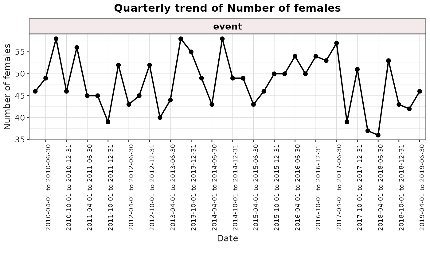
result <- summariseTrend(
  cdm = cdm,
  event = "measurement", 
  interval = "quarters",
  sex = TRUE, 
  ageGroup = list(c(0, 17), c(18, Inf)),
  dateRange = as.Date(c("2010-01-01", "2019-12-31"))
)
#> → The observation period in the cdm ends in 2019-07-03

plotTrend(
  result = result,
  colour = "sex",
  facet = "age_group"
)

When the result includes several outputs (for example, records, subjects, or person-days), select the measure to visualise with the output argument.

result <- summariseTrend(cdm,
  event = "measurement",
  interval = "quarters",
  output = c("sex", "record"),
  dateRange = as.Date(c("2010-01-01", "2019-12-31"))
)
#> → The observation period in the cdm ends in 2019-07-03
plotTrend(
  result = result,
  output = "sex"
)

You can also specify faceting with a formula or column name, and colour using one of the tidied result columns.

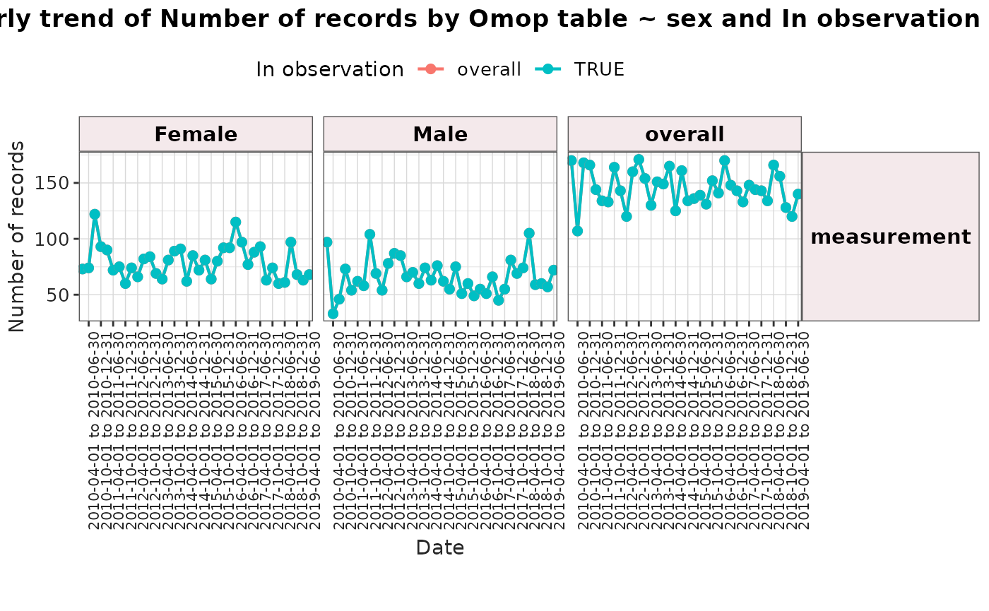
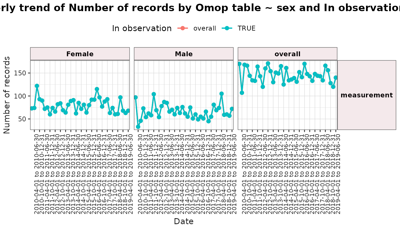
result <- summariseTrend(cdm,
  event = "measurement",
  interval = "quarters",
  sex = TRUE,
  inObservation = TRUE,
  dateRange = as.Date(c("2010-01-01", "2019-12-31"))
)
#> → The observation period in the cdm ends in 2019-07-03
plotTrend(
  result = result,
  facet = omop_table ~ sex,
  colour = "in_observation"
)

Disconnect from CDM

Finally, disconnect from the mock CDM.

cdmDisconnect(cdm = cdm)