Chapter 11 Characterization
Chapter leads: Anthony Sena & Daniel Prieto-Alhambra
Observational healthcare databases provide a valuable resource to understand variations in populations based on a host of characteristics. Characterizing populations through the use of descriptive statistics is an important first step in generating hypotheses about the determinants of health and disease. In this chapter we cover methods for characterization:
- Database-level characterization: provides a top-level set of summary statistics to understand the data profile of a database in its totality.
- Cohort characterization: describes a population in terms of its aggregate medical history.
- Treatment pathways: describes the sequence of interventions a person received for a duration of time.
- Incidence: measures the occurrence rate of an outcome in a population for a time at risk.
With the exception of database-level characterization, these methods aim to describe a population relative to an event referred to as the index date. This population of interest is defined as a cohort as described in chapter 10. The cohort defines the index date for each person in the population of interest. Using the index date as an anchor, we define the time preceding the index date as baseline time. The index date and all time after is called the post-index time.
Use-cases for characterization include disease natural history, treatment utilization and quality improvement. In this chapter will describe the methods for characterization. We will use a population of hypertensive persons to demonstrate how to use ATLAS and R to perform these characterization tasks.
11.1 Database Level Characterization
Before we can answer any characterization question about a population of interest, we must first understand the characteristics of the database we intend to utilize. Database level characterization seeks to describe the totality of a database in terms of the temporal trends and distributions. This quantitative assessment of a database will typically include questions such as:
- What is the total count of persons in this database?
- What is the distribution of age for persons?
- How long are persons in this database observed for?
- What is the proportion of persons having a {treatment, condition, procedure, etc} recorded/prescribed over time?
These database-level descriptive statistics also help a researcher to understand what data may be missing in a database. Chapter 15 goes into further detail on data quality.
11.2 Cohort Characterization
Cohort characterization describes the baseline and post-index characteristics of people in a cohort. OHDSI approaches characterization through descriptive statistics of all conditions, drug and device exposures, procedures and other clinical observations that are present in the person’s history. We also summarize the socio-demographics of members of the cohort at the index date. This approach provides a complete summary of the cohort of interest. Importantly, this enables a full exploration of the cohort with an eye towards variation in the data while also allowing for identification of potentially missing values.
Cohort characterization methods can be used for person-level drug utilization studies (DUS) to estimate the prevalence of indications and contraindications amongst users of a given treatment. The dissemination of this cohort characterization is a recommended best practice for observational studies as detailed in the Strengthening the Reporting of Observation Studies in Epidemiology (STROBE) guidelines. (Elm et al. 2008)
11.3 Treatment Pathways
Another method to characterize a population is to describe the treatment sequence during the post-index time window. For example, Hripcsak et al. (2016) utilized the OHDSI common data standards to create descriptive statistics to characterize treatment pathways for type 2 diabetes, hypertension and depression. By standardizing this analytic approach, Hripcsak and colleagues were able to run the same analysis across the OHDSI network to describe the characteristics of these populations of interest.
The pathway analysis aims to summarize the treatments (events) received by persons diagnosed with a specific condition from the first drug prescription/dispensation. In this study, treatments were described after the diagnosis of type 2 diabetes, hypertension and depression respectively. The events for each person were then aggregated to a set of summary statistics and visualized for each condition and for each database.
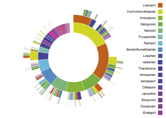
Figure 11.1: OHDSI Treatment Pathways “sunburst” visualization for hypertension
As an example, figure 11.1 represents a population of persons initiating treatment for hypertension. The first ring in the center shows the proportion of persons based on their first-line therapy. In this example, Hydrochlorothiazide is the most common first-line therapy for this population. The boxes that extend from the Hydrochlorothiazide section represent the 2nd and 3rd line therapies recorded for persons in the cohort.
A pathways analysis provides important evidence about treatment utilization amongst a population. From this analysis we can describe the most prevalent first-line therapies utilized, the proportion of persons that discontinue treatment, switch treatments or augment their therapy. Using the pathway analysis, Hripcsak et al. (2016) found that metformin is the most commonly prescribed medication for diabetes thus confirming general adoption of the first-line recommendation of the American Association of Clinical Endocrinologists diabetes treatment algorithm. Additionally, they noted that 10% of diabetes patients, 24% of hypertension patients, and 11% of depression patients followed a treatment pathway that was shared with no one else in any of the data sources.
In classic DUS terminology, treatment pathway analyses include some population-level DUS estimates such as prevalence of use of one or more medications in a specified population, as well as some person-level DUS including measures of persistence and switching between different therapies.
11.4 Incidence
Incidence rates and proportions are statistics that are used in public health to assess the occurrence of a new outcome in a population during a time-at-risk (TAR). Figure 11.2 aims to show the components of an incidence calculation for a single person:
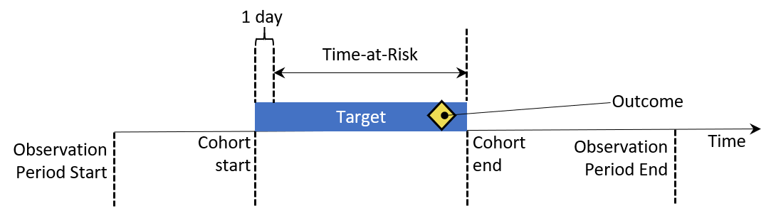
Figure 11.2: Person-level view of incidence calculation components. In this example, time-at-risk is defined to start one day after cohort start, and end at cohort end.
In figure 11.2, a person has a period of time where they are observed in the data denoted by their observation start and end time. Next, the person has a point in time where they enter and exit a cohort by meeting some eligibility criteria. The time at risk window then denotes when we seek to understand the occurrence of an outcome. If the outcome falls into the TAR, we count that as an incidence of the outcome.
There are two metrics for calculating incidence:
\[ Incidence\;Proportion = \frac{\#\;persons\;in\;cohort\;with\;new\;outcome\;during\;TAR}{\#\;persons\;in\;cohort\;with\;TAR} \]
An incidence proportion provides a measure of the new outcomes per person in the population during the time-at-risk. Stated another way, this is the proportion of the population of interest that developed the outcome in a defined timeframe.
\[ Incidence\;Rate = \frac{\#\;persons\;in\;cohort\;with\;new\;outcome\;during\;TAR}{person\;time\;at\;risk\;contributed\;by\;persons\;in\;cohort} \]
An incidence rate is a measure of the number of new outcomes during the cumulative TAR for the population. When a person experiences the outcome in the TAR, their contribution to the total person-time stops at the occurrence of the outcome event. The cumulative TAR is referred to as person-time and is expressed in days, months or years.
When calculated for therapies, incidence proportions and incidence rates of use of a given therapy are classic population-level DUS.
11.5 Characterizing Hypertensive Persons
Per the World Health Organization’s (WHO) global brief on hypertension (Who 2013), there are significant health and economic gains attached to early detection, adequate treatment and good control of hypertension. The WHO brief provides an overview of hypertension and characterizes the burden of the disease across different countries. The WHO provides descriptive statistics around hypertension for geographic regions, socio-economic class and gender.
Observational data sources provide a way to characterize hypertensive populations as was done by the WHO. In the subsequent sections of this chapter, we’ll explore the ways that we make use of ATLAS and R to explore a database to understand its composition for studying hypertensive populations. Then, we will use these same tools to describe the natural history and treatment patterns of hypertensive populations.
11.6 Database Characterization in ATLAS
Here we demonstrate how to use the data sources module in ATLAS to explore database characterization statistics created with ACHILLES to find database level characteristics related to hypertensive persons. Start by clicking on  in the left bar of ATLAS to start. In the first drop down list shown in ATLAS, select the database to explore. Next, use the drop down below the database to start exploring reports. To do this, select the Condition Occurrence from the report drop down which will reveal a treemap visualization of all conditions present in the database:
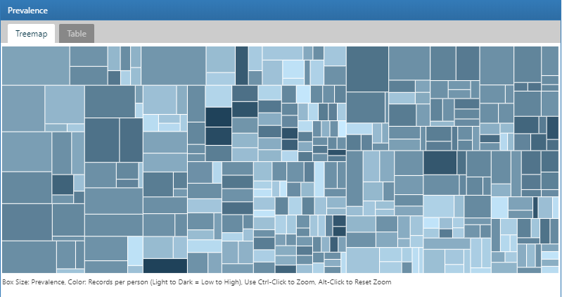
Figure 11.3: Atlas Data Sources: Condition Occurrence Treemap
To search for a specific condition of interest, click on the Table tab to reveal the full list of conditions in the database with person count, prevalence and records per person. Using the filter box on the top, we can filter down the entries in the table based on concept name containing the term “hypertension”:

Figure 11.4: Atlas Data Sources: Conditions with “hypertension” found in the concept name
We can explore a detailed drill-down report of a condition by clicking on a row. In this case, we will select “essential hypertension” to get a breakdown of the trends of the selected condition over time and by gender, the prevalence of the condition by month, the type recorded with the condition and the age at first occurrence of the diagnosis:
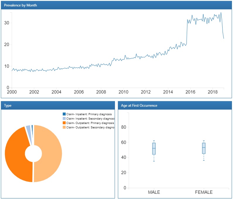
Figure 11.5: Atlas Data Sources: Essential hypertension drill down report
Now that we have reviewed the database’s characteristics for the presence of hypertension concepts and the trends over time, we can also explore drugs used to treat hypertensive persons. The process to do this follows the same steps except we use the Drug Era report to review characteristics of drugs summarized to their RxNorm Ingredient. Once we have explored the database characteristics to review items of interest, we are ready to move forward with constructing cohorts to identify the hypertensive persons to characterize.
11.7 Cohort Characterization in ATLAS
Here we demonstrate how to use ATLAS to perform large-scale cohort characterization for several cohorts. Click on the 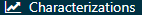 in the left bar of ATLAS and create a new characterization analysis. Give the analysis a name a save using the
  button.
11.7.1 Design
A characterization analysis requires at least one cohort and at least one feature to characterize. For this example, we will use two cohorts. The first cohort will define persons initiating a treatment for hypertension as their index date with at least one diagnosis of hypertension in the year prior. We will also require that persons in this cohort have at least one year of observation after initiating the hypertensive drug (Appendix B.6). The second cohort is identical to the first cohort described with a requirement having at least three years of observation instead of one (Appendix B.7).
Cohort Definitions
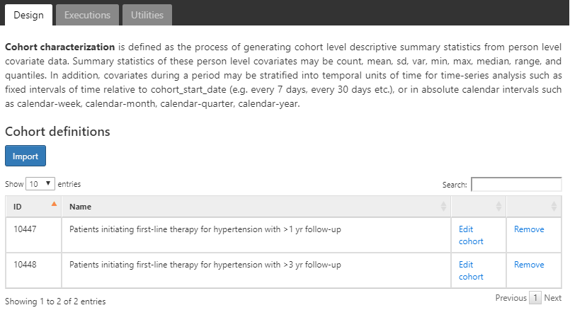
Figure 11.6: Characterization design tab - cohort definition selection
We assume the cohorts have already been created in ATLAS as described in Chapter 10. Click on  and select the cohorts as shown in figure 11.6. Next, we’ll define the features to use for characterizing these two cohorts.
Feature Selection
ATLAS comes with nearly 100 preset feature analyses that are used to perform characterization across the clinical domains modeled in the OMOP CDM. Each of these preset feature analyses perform aggregation and summarization functions on clinical observations for the selected target cohorts. These calculations provide potentially thousands of features to describe the cohorts baseline and post-index characteristics. Under the hood, ATLAS is utilizing the OHDSI FeatureExtraction R package to perform the characterization for each cohort. We will cover the use of FeatureExtraction and R in more detail in the next section.
Click on to select the feature to characterize. Below is a list of features we will use to characterize these cohorts:
Figure 11.7: Characterization design tab - feature selection.
The figure above shows the list of features selected along with a description of what each feature will characterize for each cohort. The features that start with the name “Demographics” will calculate the demographic information for each person at the cohort start date. For the features that start with a domain name (i.e. Visit, Procedure, Condition, Drug, etc), these will characterize all recorded observations in that domain. Each domain feature has four options of time window preceding the cohort star, namely:
- Any time prior: uses all available time prior to cohort start that fall into the person’s observation period
- Long term: 365 days prior up to and including the cohort start date.
- Medium term: 180 days prior up to and including the cohort start date.
- Short term: 30 days prior up to and including the cohort start date.
Subgroup Analysis
What if we were interested in creating different characteristics based on gender? We can use the “subgroup analyses” section to define new subgroups of interest to use in our characterization.
To create a subgroup, click on and add your criteria for subgroup membership. This step is similar to the criteria used to identify cohort enrollment. In this example, we’ll define a set of criteria to identify females amongst our cohorts:
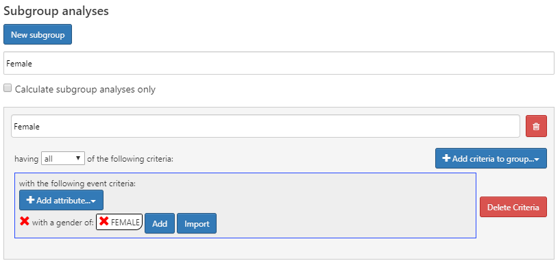
Figure 11.8: Characterization design with female sub group analysis.
11.7.2 Executions
Once we have our characterization designed, we can execute this design against one or more databases in our environment. Navigate to the Executions tab and click on the Generate button to start the analysis on a database:
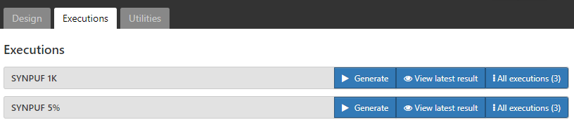
Figure 11.9: Characterization design execution - CDM source selection.
Once the analysis is complete, we can view reports by clicking on the “All Executions” button and from the list of executions, select “View Reports”. Alternatively, you can click “View latest result” to view the last execution performed.
11.7.3 Results
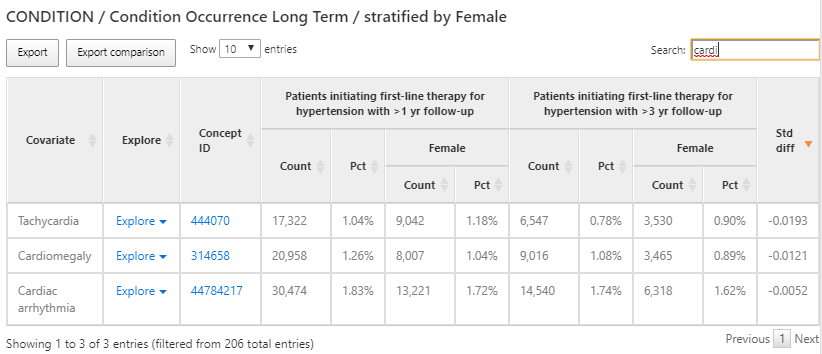
Figure 11.10: Characterization results - condition occurrence long term.
The results provide a tabular view of the different features for each cohort selected in the design. In figure 11.10, a table provides a summary of all conditions present in the two cohorts in the preceding 365 days from the cohort start. Each covariate has a count and percentage for each cohort and the female subgroup we defined within each cohort.
We used the search box to filter the results to see what proportion of persons have a cardiac arrhythmia in their history in an effort to understand what cardiovascular-related diagnoses are observed in the populations. We can use the Explore link next to the cardiac arrhythmia concept to open a new window with more details about the concept for a single cohort as shown in figure 11.11:
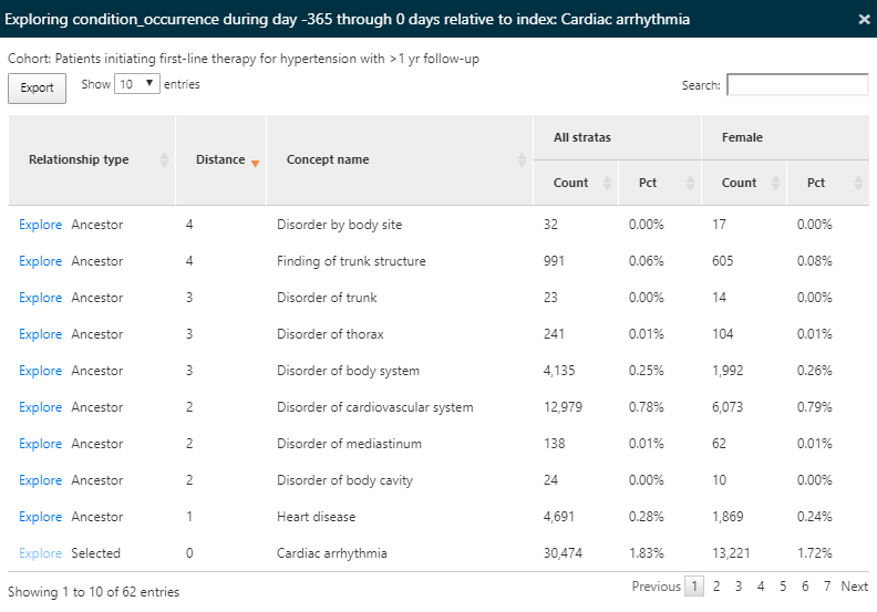
Figure 11.11: Characterization results - exploring a single concept.
Since we have characterized all condition concepts for our cohorts, the explore option enables a view of all ancestor and descendant concepts for the selected concept, in this case cardiac arrhythmia. This exploration allows us to navigate the hierarchy of concepts to explore other cardiac diseases that may appear for our hypertensive persons. Like in the summary view, the count and percentage are displayed.
We can also use the same characterization results to find conditions that are contraindicated for some anti-hypertensive treatment such as angioedema. To do this, we’ll follow the same steps above but this time search for ‘edema’ as shown in figure 11.12:
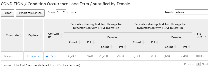
Figure 11.12: Characterization results - exploring a contraindicated condition.
Once again, we’ll use the explore feature to see the characteristics of Edema in the hypertension population to find the prevalence of angioedema:
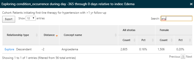
Figure 11.13: Characterization results - exploring a contraindicated condition details.
Here we find that a portion of this population has a record of angioedema in the year prior to starting an anti-hypertensive medication.
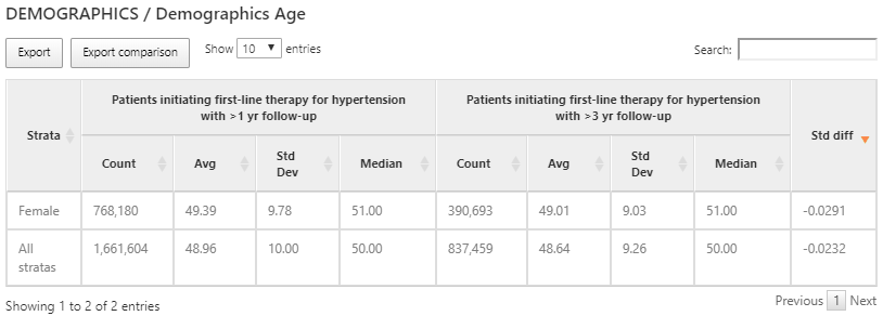
Figure 11.14: Characterization results of age for each cohort and sub group.
While domain covariates are computed using a binary indicator (i.e. was a record of the code present in the prior timeframe), some variables provide a continuous value such as the age of persons at cohort start. In the example above, we show the age for the 2 cohorts characterized expressed with the count of persons, mean age, median age and standard deviation.
11.7.4 Defining Custom Features
In addition to the preset features, ATLAS supports the ability to allow for user-defined custom features. To do this, click the Characterization left-hand menu item, then click the Feature Analysis tab and click the New Feature Analysis button. Provide a name for the custom feature and save it using the button.
In this example, we will define a custom feature that will identify the count of persons in each cohort that have a drug era of ACE inhibitors in their history after cohort start:
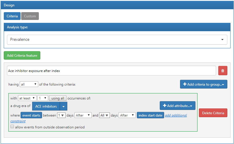
Figure 11.15: Custom feature definition in ATLAS.
The criteria defined above assumes that it will be applied to a cohort start date. Once we have defined the criteria and saved it, we can apply it to the characterization design we created in the previous section. To do this, open the characterization design and navigate to the Feature Analysis section. Click the button and from the menu select the new custom features. They will now appear in the feature list for the characterization design. As described earlier, we can execute this design against a database to produce the characterization for this custom feature:
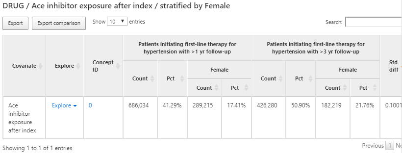
Figure 11.16: Custom feature results display.
11.8 Cohort Characterization in R
We may also choose to characterize cohorts using R. Here we’ll describe how to use the OHDSI R package FeatureExtraction to generate baseline features (covariates) for our hypertension cohorts. FeatureExtraction provides users with the ability to construct covariates in three ways:
- Choose the default set of covariates
- Choose from a set of pre-specified analyses
- Create a set of custom analyses
FeatureExtraction creates covariates in two distinct ways: person-level features and aggregate features. Person-level features are useful for machine learning applications. In this section, we’ll focus on using aggregate features that are useful for generating baseline covariates that describe the cohort of interest. Additionally, we’ll focus on the second two ways of constructing covariates: pre-specified and custom analyses and leave using the default set as an exercise for the reader.
11.8.1 Cohort Instantiation
We first need to instantiate the cohort to characterize it. Instantiating cohorts is described in Chapter 10. In this example, we’ll use the persons initiating a first-line therapy for hypertension with 1 year follow up (Appendix B.6). We leave characterizing the other cohorts in Appendix B as an exercise for the reader. We will assume the cohort has been instantiated in a table called scratch.my_cohorts with cohort definition ID equal to 1.
11.8.2 Data Extraction
We first need to tell R how to connect to the server. FeatureExtraction uses the DatabaseConnector package, which provides a function called createConnectionDetails. Type ?createConnectionDetails for the specific settings required for the various database management systems (DBMS). For example, one might connect to a PostgreSQL database using this code:
library(FeatureExtraction)
connDetails <- createConnectionDetails(dbms = "postgresql",
                                       server = "localhost/ohdsi",
                                       user = "joe",
                                       password = "supersecret")

cdmDbSchema <- "my_cdm_data"
cohortsDbSchema <- "scratch"
cohortsDbTable <- "my_cohorts"
cdmVersion <- "5"
The last four lines define the cdmDbSchema, cohortsDbSchema, and cohortsDbTable variables, as well as the CDM version. We will use these later to tell R where the data in CDM format live, where the cohorts of interest have been created, and what version CDM is used. Note that for Microsoft SQL Server, database schemas need to specify both the database and the schema, so for example cdmDbSchema <- "my_cdm_data.dbo".
11.8.3 Using Prespecified Analyses
The function createCovariateSettings allow the user to choose from a large set of predefined covariates. Type ?createCovariateSettings to get an overview of the available options. For example:
settings <- createCovariateSettings(
  useDemographicsGender = TRUE,
  useDemographicsAgeGroup = TRUE,
  useConditionOccurrenceAnyTimePrior = TRUE)
This will create binary covariates for gender, age (in 5 year age groups), and each concept observed in the condition_occurrence table any time prior to (and including) the cohort start date.
Many of the prespecified analyses refer to a short, medium, or long term time window. By default, these windows are defined as:
- Long term: 365 days prior up to and including the cohort start date.
- Medium term: 180 days prior up to and including the cohort start date.
- Short term: 30 days prior up to and including the cohort start date.
However, the user can change these values. For example:
settings <- createCovariateSettings(useConditionEraLongTerm = TRUE,
                                    useConditionEraShortTerm = TRUE,
                                    useDrugEraLongTerm = TRUE,
                                    useDrugEraShortTerm = TRUE,
                                    longTermStartDays = -180,
                                    shortTermStartDays = -14,
                                    endDays = -1)
This redefines the long-term window as 180 days prior up to (but not including) the cohort start date, and redefines the short term window as 14 days prior up to (but not including) the cohort start date.
Again, we can also specify which concept IDs should or should not be used to construct covariates:
settings <- createCovariateSettings(useConditionEraLongTerm = TRUE,
                                    useConditionEraShortTerm = TRUE,
                                    useDrugEraLongTerm = TRUE,
                                    useDrugEraShortTerm = TRUE,
                                    longTermStartDays = -180,
                                    shortTermStartDays = -14,
                                    endDays = -1,
                                    excludedCovariateConceptIds = 1124300,
                                    addDescendantsToExclude = TRUE,
aggregated = TRUE)aggregated = TRUE for all of the examples above indicate to FeatureExtraction to provide summary statistics. Excluding this flag will compute covariates for each person in the cohort.
11.8.4 Creating Aggregated Covariates
The following code block will generate aggregated statistics for a cohort:
covariateSettings <- createDefaultCovariateSettings()

covariateData2 <- getDbCovariateData(
  connectionDetails = connectionDetails,
  cdmDatabaseSchema = cdmDatabaseSchema,
  cohortDatabaseSchema = resultsDatabaseSchema,
  cohortTable = "cohorts_of_interest",
  cohortId = 1,
  covariateSettings = covariateSettings,
  aggregated = TRUE)

summary(covariateData2)
And the output will look similar to the following:
## CovariateData Object Summary
##
## Number of Covariates: 41330
## Number of Non-Zero Covariate Values: 41330
11.8.5 Output Format
The two main components of the aggregated covariateData object are covariates and covariatesContinuous for binary and continuous covariates respectively:
11.8.6 Custom Covariates
FeatureExtraction also provides the ability to define and utilize custom covariates. These details are an advanced topic and covered in the user documentation: http://ohdsi.github.io/FeatureExtraction/.
11.9 Cohort Pathways in ATLAS
The goal with a pathway analysis is to understand the sequencing of treatments along in one or more cohorts of interest. The methods applied are based on the design reported by Hripcsak et al. (2016). These methods were generalized and codified into a feature called Cohort Pathways in ATLAS.
Cohort pathways aims to provide analytic capabilities to summarize the events following the cohort start date of one or more target cohorts. To do this, we create a set of cohorts to identify the clinical events of interest for the target population called event cohort. Focusing on how this might look for a person in the target cohort:
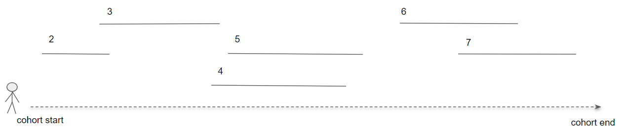
Figure 11.17: Pathways analysis in the context of a single person.
In figure 11.17, the person is part of the target cohort with a defined start and end date. Then, the numbered line segments represent where that person also is identified in an event cohort for a duration of time. Event cohorts allow us to describe any clinical event of interest that is represented in the CDM such that we are not constrained to creating a pathway for a single domain or concept.
To start, click on  in the left bar of ATLAS to create a new cohort pathways study. Provide a descriptive name and press the save button.
11.9.1 Design
To start, we will continue to use the cohorts initiating a first-line therapy for hypertension with 1 and 3 years follow up (Appendix B.6, B.7). Use the button to import the 2 cohorts.
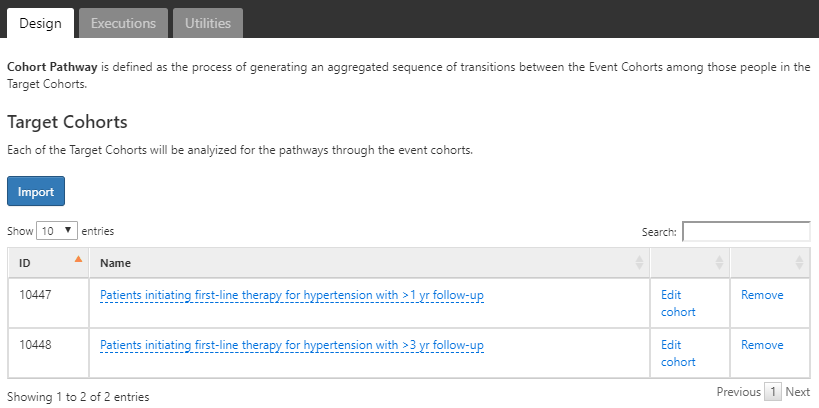
Figure 11.18: Pathways analysis with target cohorts selected.
Next we’ll define the event cohorts by creating a cohort for each first-line hypertensive drug of interest. For this, we’ll start by creating a cohort of ACE inhibitor users and define the cohort end date as the end of continuous exposure. We’ll do the same for 8 other hypertensive medications and note that these definitions are found in Appendix B.8-B.16. Once complete use the button to import these into the Event Cohort section of the pathway design:
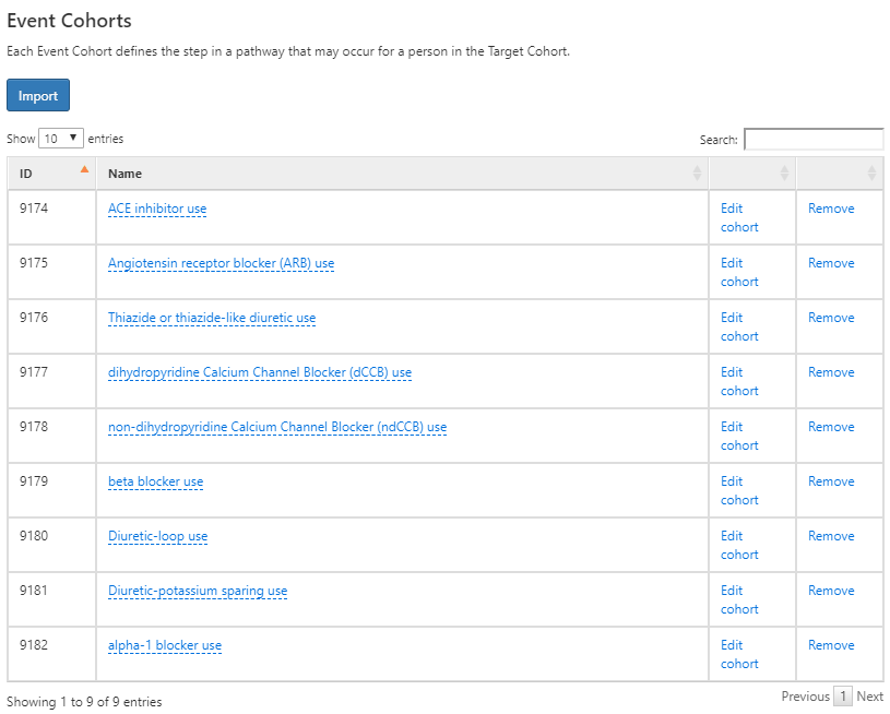
Figure 11.19: Event cohorts for pathway design for initiating a first-line antihypertensive therapy.
When complete, your design should look like the one above. Next, we’ll need to decide on a few additional analysis settings:
- Combination window: This setting allows you to define a window of time, in days, in which overlap between events is considered a combination of events. For example, if two drugs represented by 2 event cohorts (event cohort 1 and event cohort 2) overlap within the combination window the pathways algorithm will combine them into “event cohort 1 + event cohort 2”.
- Minimum cell count: Event cohorts with less than this number of people will be censored (removed) from the output to protect privacy.
- Max path length: This refers to the maximum number of sequential events to consider for the analysis.
11.9.2 Executions
Once we have our pathway analysis designed, we can execute this design against one or more databases in our environment. This works the same way as we described for cohort characterization in ATLAS. Once complete, we can review the results of the analysis.
11.9.3 Viewing Results
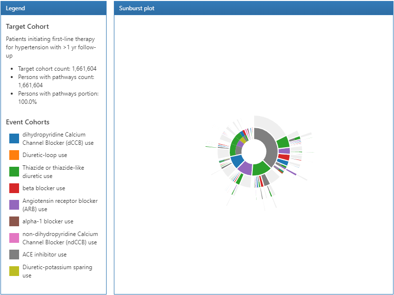
Figure 11.20: Pathways results legend and sunburst visualization.
The results of a pathway analysis are broken into 3 sections: The legend section displays the total number of persons in the target cohort along with the number of persons that had 1 or more events in the pathway analysis. Below that summary are the color designations for each of the cohorts that appear in the sunburst plot in the center section.
The sunburst plot is a visualization that represents the various event pathways taken by persons over time. The center of the plot represents the cohort entry and the first color-coded ring shows the proportion of persons in each event cohort. In our example, the center of the circle represents hypertensive persons initiating a first line therapy. Then, the first ring in the sunburst plot shows the proportion of persons that initiated a type of first-line therapy defined by the event cohorts (i.e. ACE inhibitors, Angiotensin receptor blockers, etc). The second set of rings represents the 2nd event cohort for persons. In certain event sequences, a person may never have a 2nd event cohort observed in the data and that proportion is represented by the grey portion of the ring.
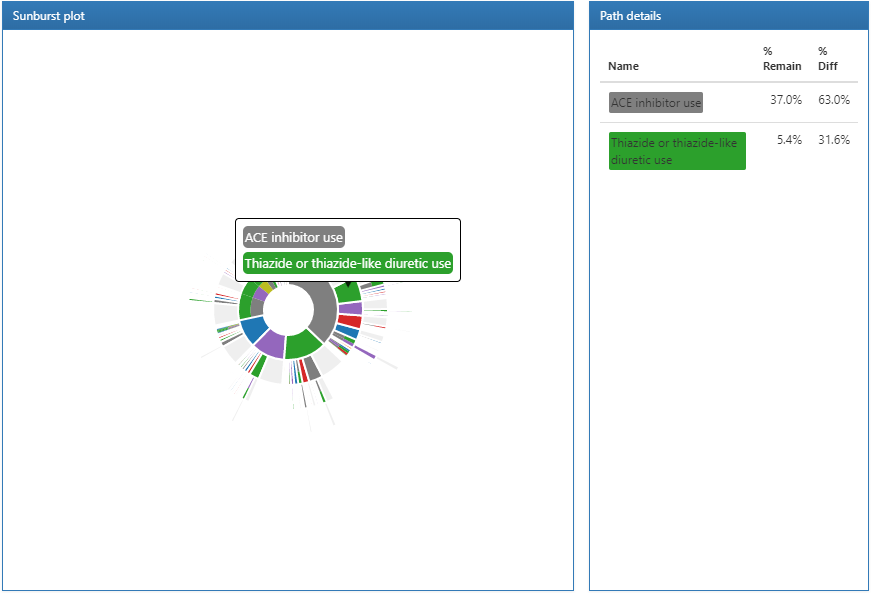
Figure 11.21: Pathways results displaying path details.
Clicking on a section of the sunburst plot will display the path details on the right. Here we can see that the largest proportion of people in our target cohort initiated a first-line therapy with ACE inhibitors and from that group, a smaller proportion started a Thiazide or thiazide diuretics.
11.10 Incidence Analysis in ATLAS
In an incidence calculation, we describe: amongst the persons in the target cohort, who experienced the outcome cohort during the time at risk period. Here we will design an incidence analysis to characterize angioedema and acute myocardial infarction outcomes amongst new users of ACE inhibitors (ACEi) and Thiazides and thiazide-like diuretics (THZ). We will assess these outcomes during the TAR that a person was exposed to the drug. Additionally, we will add an outcome of drug exposure to Angiotensin receptor blockers (ARBs) to measure the incidence of new use of ARBs during exposure to the target cohorts (ACEi and THZ). This outcome definition provides an understanding of how ARBs are utilized amongst the target populations.
To start, click on 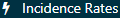 in the left bar of ATLAS to create a new incidence analysis. Provide a descriptive name and press the save button .
11.10.1 Design
We assume the cohorts used in this example have already been created in ATLAS as described in Chapter 10. The Appendix provides the full definitions of the target cohorts (Appendix B.2, B.5), and outcomes (Appendix B.4, B.3, B.9) cohorts.
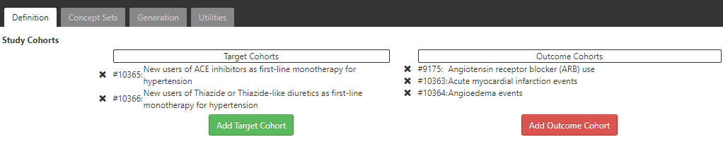
Figure 11.22: Incidence Rate target and outcome definition.
On the definition tab, click to choose the New users of ACE inhibitors cohort and the New users of Thiazide or Thiazide-like diuretics cohort. Close the dialog to view that these cohorts are added to the design. Next we add our outcome cohorts by clicking on and from the dialog box, select the outcome cohorts of acute myocardial infarction events, angioedema events and Angiotensin receptor blocker (ARB) use. Again, close the window to view that these cohorts are added to the outcome cohorts section of the design.
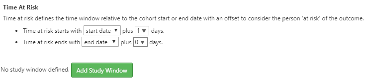
Figure 11.23: Incidence Rate target and outcome definition.
Next, we will define the time at risk window for the analysis. As shown above, the time at risk window is defined relative to the cohort start and end dates. Here we will define the time at risk start as 1 day after cohort start for our target cohorts. Next, we’ll define the time at risk to end at the cohort end date. In this case, the definition of the ACEi and THZ cohorts have a cohort end date when the drug exposure ends.
ATLAS also provides a way to stratify the target cohorts as part of the analysis specification:
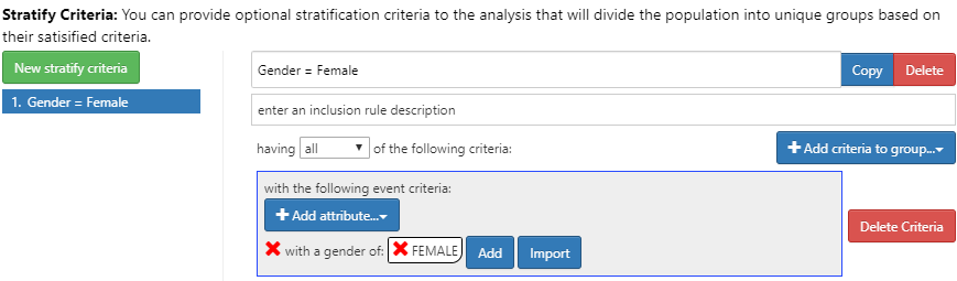
Figure 11.24: Incidence Rate strata definition for females.
To do this, click the New Stratify Criteria button and follow the same steps described in Chapter 11. Now that we have completed the design, we can move to executing our design against one or more databases.
11.10.2 Executions
Click the Generation tab and then the  button to reveal a list of databases to use to execute the analysis:
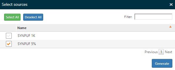
Figure 11.25: Incidence Rate analysis execution.
Select one or more databases and click the Generate button to start the analysis to analyze all combinations of targets and outcomes specified in the design.
11.10.3 Viewing Results
On the Generation tab, the top portion of the screen allows you to select a target and outcome to use when viewing the results. Just below this a summary of the incidence is shown for each database used in the analysis.
Select the target cohort of ACEi users and the Acute Myocardial Infarction (AMI) from the respective dropdown lists. Click the  button to reveal the incidence analysis results:
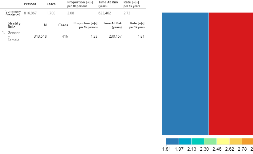
Figure 11.26: Incidence Rate analysis output - New ACEi users with AMI outcome.
A summary for the database shows the total persons in the cohort that were observed during the TAR along with the total number of cases. The proportion shows the number of cases per 1000 people. The time at risk, in years, is calculated for the target cohort. The incidence rate is expressed as the number of cases per 1000 person-years.
We can also view the incidence metrics for the strata that we defined in the design. The same metrics mentioned above are calculated for each stratum. Additionally, a treemap visualization provides a representation of the proportion of each stratum represented by the boxed areas. The color represents the incidence rate as shown in the scale along the bottom.
We can gather the same information to see the incidence of new use of ARBs amongst the ACEi population. Using the dropdown at the top, change the outcome to ARBs use and click the button to reveal the details.
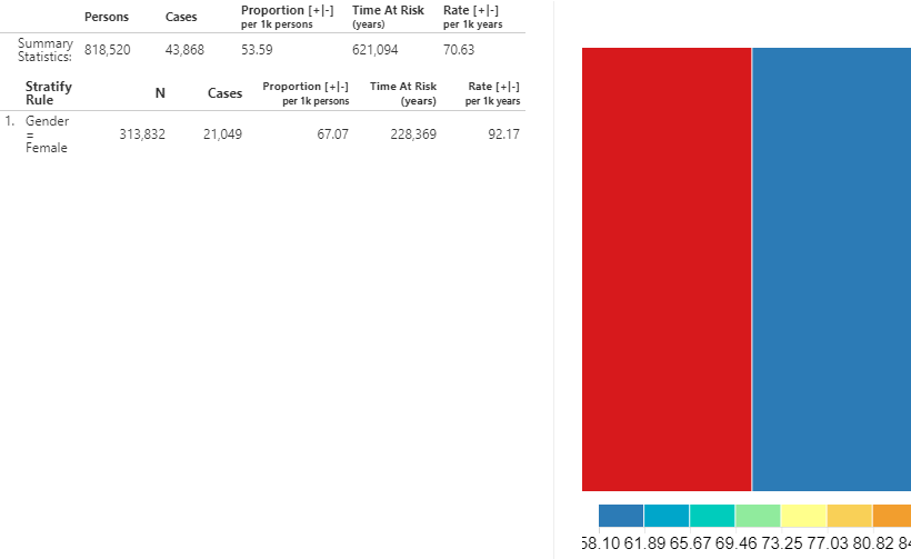
Figure 11.27: Incidence Rate - New users of ACEi receiving ARBs treatment during ACEi exposure.
As shown, the metrics calculated are the same but the interpretation is different since the input (ARB use) references a drug utilization estimate instead of a health outcome.
11.11 Summary
OHDSI offers tools to characterize an entire database, or a cohort of interest.
Cohort characterization describes a cohort of interest during the time preceding the index date (baseline) and the time after index (post-index).
ATLAS’s characterization module and the OHDSI Methods Library provide the capability to calculate baseline characteristics for multiple time windows.
ATLAS’s pathways and incidence rate modules provide descriptive statistics during the post-index time period.
11.12 Exercises
Prerequisites
For these exercises, access to an ATLAS instance is required. You can use the instance at http://atlas-demo.ohdsi.org, or any other instance you have access to.
Exercise 11.1 We would like to understand how celecoxib is used in the real world. To start, we would like to understand what data a database has on this drug. Use the ATLAS Data Sources module to find information on celecoxib.
Exercise 11.2 We would like to better understand the disease natural history of celecoxib users. Create a simple cohort of new users of celecoxib using a 365-day washout period (see Chapter 10 for details on how to do this), and use ATLAS to create a characterization of this cohort, showing co-morbid conditions and drug-exposures.
Exercise 11.3 We are interested in understand how often gastrointestinal (GI) bleeds occur any time after people initiate celecoxib treatment. Create a cohort of GI bleed events, simply defined as any occurrence of concept 192671 (“Gastrointestinal hemorrhage”) or any of its descendants. Compute the incidence rate of these GI events after celecoxib initiation, using the exposure cohort defined in the previous exercise.
Suggested answers can be found in Appendix E.7.
References
Elm, Erik von, Douglas G. Altman, Matthias Egger, Stuart J. Pocock, Peter C. Gøtzsche, and Jan P. Vandenbroucke. 2008. “The Strengthening the Reporting of Observational Studies in Epidemiology (Strobe) Statement: Guidelines for Reporting Observational Studies.” Journal of Clinical Epidemiology 61 (4): 344–49. https://doi.org/10.1016/j.jclinepi.2007.11.008.
Hripcsak, George, Patrick B. Ryan, Jon D. Duke, Nigam H. Shah, Rae Woong Park, Vojtech Huser, Marc A. Suchard, et al. 2016. “Characterizing treatment pathways at scale using the OHDSI network.” Proceedings of the National Academy of Sciences 113 (27): 7329–36. https://doi.org/10.1073/pnas.1510502113.
Who, A. 2013. “Global Brief on Hypertension.” World Health Organization. https://www.who.int/cardiovascular_diseases/publications/global_brief_hypertension/en/.