Chapter 6 Extract Transform Load
Chapter leads: Clair Blacketer & Erica Voss
6.1 Introduction
In order to get from the native/raw data to the OMOP Common Data Model (CDM) we have to create an extract, transform, and load (ETL) process. This process should restructure the data to the CDM, and add mappings to the Standardized Vocabularies, and is typically implemented as a set of automated scripts, for example SQL scripts. It is important that this ETL process is repeatable, so that it can be rerun whenever the source data is refreshed.
Creating an ETL is usually a large undertaking. Over the years, we have developed best practices, consisting of four major steps:
- Data experts and CDM experts together design the ETL.
- People with medical knowledge create the code mappings.
- A technical person implements the ETL.
- All are involved in quality control.
In this chapter we will discuss each of these steps in detail. Several tools have been developed by the OHDSI community to support some of these steps, and these will be discussed as well. We close this chapter with a discussion of CDM and ETL maintenance.
6.2 Step 1: Design the ETL
It is important to clearly separate the design of the ETL from the implementation of the ETL. Designing the ETL requires extensive knowledge of both the source data, as well as the CDM. Implementing the ETL on the other hand typically relies mostly on technical expertise on how to make the ETL computationally efficient. If we try to do both at once, we are likely to get stuck in nitty-gritty details, while we should be focusing on the overall picture.
Two closely-integrated tools have been developed to support the ETL design process: White Rabbit, and Rabbit-in-a-Hat.
6.2.1 White Rabbit
To initiate an ETL process on a database you need to understand your data, including the tables, fields, and content. This is where the White Rabbit tool comes in. White Rabbit is a software tool to help prepare for ETLs of longitudinal healthcare databases into the OMOP CDM. White Rabbit scans your data and creates a report containing all the information necessary to begin designing the ETL. All source code and installation instructions, as well as a link to the manual, are available on GitHub.30
Scope and Purpose
White Rabbit’s main function is to perform a scan of the source data, providing detailed information on the tables, fields, and values that appear in a field. The source data can be in comma-separated text files, or in a database (MySQL, SQL Server, Oracle, PostgreSQL, Microsoft APS, Microsoft Access, Amazon Redshift). The scan will generate a report that can be used as a reference when designing the ETL, for instance by using it in conjunction with the Rabbit-In-a-Hat tool. White Rabbit differs from standard data profiling tools in that it attempts to prevent the display of personally identifiable information (PII) data values in the generated output data file.
Process Overview
The typical sequence for using the software to scan source data:
- Set working folder, the location on the local desktop computer where results will be exported.
- Connect to the source database or CSV text file and test connection.
- Select the tables of interest for the scan and scan the tables.
- White Rabbit creates an export of information about the source data.
Setting a Working Folder
After downloading and installing the White Rabbit application, the first thing you need to do is set a working folder. Any files that White Rabbit creates will be exported to this local folder. Use the “Pick Folder” button shown in Figure 6.1 to navigate in your local environment where you would like the scan document to go.
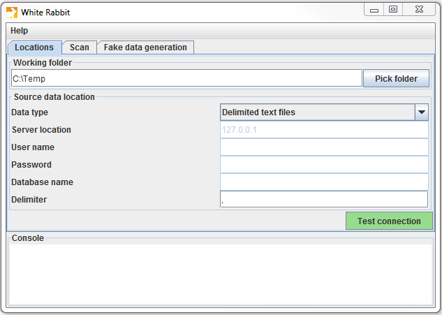
Figure 6.1: The “Pick Folder” button allows the specification of a working folder for the White Rabbit application.
Connection to a Database
White Rabbit supports delimited text files and various database platforms. Hover the mouse over the various fields to get a description of what is required. More detailed information can be found in the manual.
Scanning the Tables in a Database
After connecting to a database, you can scan the tables contained therein. A scan generates a report containing information on the source data that can be used to help design the ETL. Using the Scan tab shown in Figure 6.2 you can either select individual tables in the selected source database by clicking on “Add” (Ctrl + mouse click), or automatically select all tables in the database by clicking on “Add all in DB”.
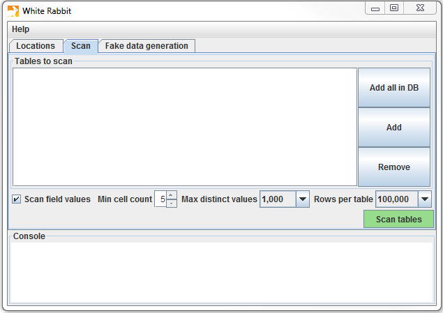
Figure 6.2: White Rabbit Scan tab.
There are a few setting options as well with the scan:
- Checking the “Scan field values” tells WhiteRabbit that you would like to investigate which values appear in the columns.
- “Min cell count” is an option when scanning field values. By default, this is set to 5, meaning values in the source data that appear less than 5 times will not appear in the report. Individual data sets may have their own rules about what this minimum cell count can be.
- “Rows per table” is an option when scanning field values. By default, White Rabbit will scan 100,000 randomly selected rows in the table.
Once all settings are completed, press the “Scan tables” button. After the scan is completed the report will be written to the working folder.
Interpreting the Scan Report
Once the scan is complete, an Excel file is generated in the selected folder with one tab present for each table scanned as well as an overview tab. The overview tab lists all tables scanned, each field in each table, the data type of each field, the maximum length of the field, the number of rows in the table, the number of rows scanned, and how often each field was found to be empty. Figure 6.3. shows an example overview tab.
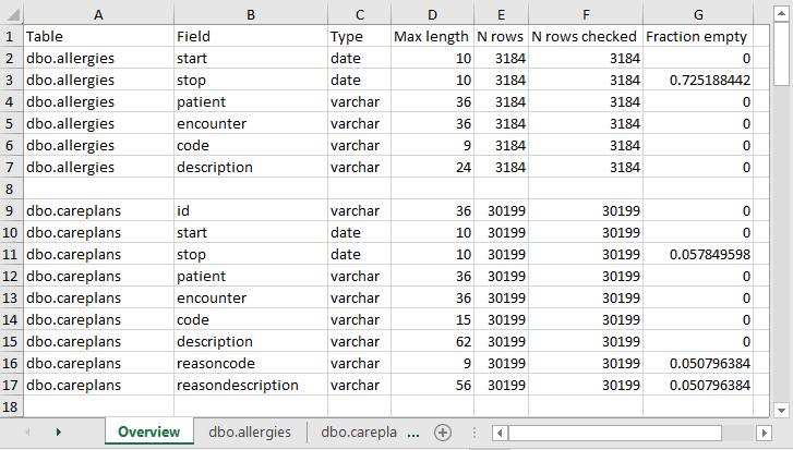
Figure 6.3: Example overview tab from a scan report.
The tabs for each of the tables show each field, the values in each field, and the frequency of each value. Each source table column will generate two columns in the Excel. One column will list all distinct values that have a “Min cell count” greater than what was set at time of the scan. If a list of unique values was truncated, the last value in the list will be “List truncated”; this indicates that there are one or more additional unique source values that appear less than the number entered in the “Min cell count”. Next to each distinct value will be a second column that contains the frequency (the number of times that value occurs in the sample). These two columns (distinct values and frequency) will repeat for all the source columns in the table profiled in the workbook.
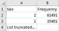
Figure 6.4: Example values for a single column.
The report is powerful in understanding your source data by highlighting what exists. For example, if the results shown in Figure 6.4 were given back on the “Sex” column within one of the tables scanned, we can see that there were two common values (1 and 2) that appeared 61,491 and 35,401 times respectively. White Rabbit will not define 1 as male and 2 as female; the data holder will typically need to define source codes unique to the source system. However, these two values (1 & 2) are not the only values present in the data because we see this list was truncated. These other values appear with very low frequency (defined by “Min cell count”) and often represent incorrect or highly suspicious values. When generating an ETL we should not only plan to handle the high-frequency gender concepts 1 and 2 but the other low-frequency values that exist within this column. For example, if those lower frequency genders were “NULL” we want to make sure the ETL can handle processing that data and knows what to do in that situation.
6.2.2 Rabbit-In-a-Hat
With the White Rabbit scan in hand, we have a clear picture of the source data. We also know the full specification of the CDM. Now we need to define the logic to go from one to the other. This design activity requires thorough knowledge of both the source data and the CDM. The Rabbit-in-a-Hat tools that comes with the White Rabbit software is specifically designed to support a team of experts in these areas. In a typical setting, the ETL design team sits together in a room, while Rabbit-in-a-Hat is projected on a screen. In a first round, the table-to-table mappings can be collaboratively decided, after which field-to-field mappings can be designed, while defining the logic by which values will be transformed.
Scope and Purpose
Rabbit-In-a-Hat is designed to read and display a White Rabbit scan document. White Rabbit generates information about the source data while Rabbit-In-a-Hat uses that information and through a graphical user interface to allow a user to connect source data to tables and columns within the CDM. Rabbit-In-a-Hat generates documentation for the ETL process, it does not generate code to create an ETL.
Process Overview
The typical sequence for using this software to generate documentation of an ETL:
- Scanned results from WhiteRabbit completed.
- Open scanned results; interface displays source tables and CDM tables.
- Connect source tables to CDM tables where the source table provides information for that corresponding CDM table.
- For each source table to CDM table connection, further define the connection with source column to CDM column detail.
- Save Rabbit-In-a-Hat work and export to a MS Word document.
Writing ETL Logic
Once you have opened your White Rabbit scan report in Rabbit-In-a-Hat you are ready to begin designing and writing the logic for how to convert the source data to the OMOP CDM. As an example, the next few sections will depict how some of the tables in the Synthea31 database might look during conversion.
General Flow of an ETL
Since the CDM is a person-centric model it is always a good idea to start mapping the PERSON table first. Every clinical event table (CONDITION_OCCURRENCE, DRUG_EXPOSURE, PROCEDURE_OCCURRENCE, etc.) refers to the PERSON table by way of the person_id so working out the logic for the PERSON table first makes it easier later on. After the PERSON table a good rule of thumb is to convert the OBSERVATION_PERIOD table next. Each person in a CDM database should have at least one OBSERVATION_PERIOD and, generally, most events for a person fall within this timeframe. Once the PERSON and OBSERVATION_PERIOD tables are done the dimensional tables like PROVIDER, CARE_SITE, and LOCATION are typically next. The final table logic that should be worked out prior to the clinical tables is VISIT_OCCURRENCE. Often this is the most complicated logic in the entire ETL and it is some of the most crucial since most events that occur during the course of a person’s patient journey will happen during visits. Once those tables are finished it is your choice which CDM tables to map and in which order.
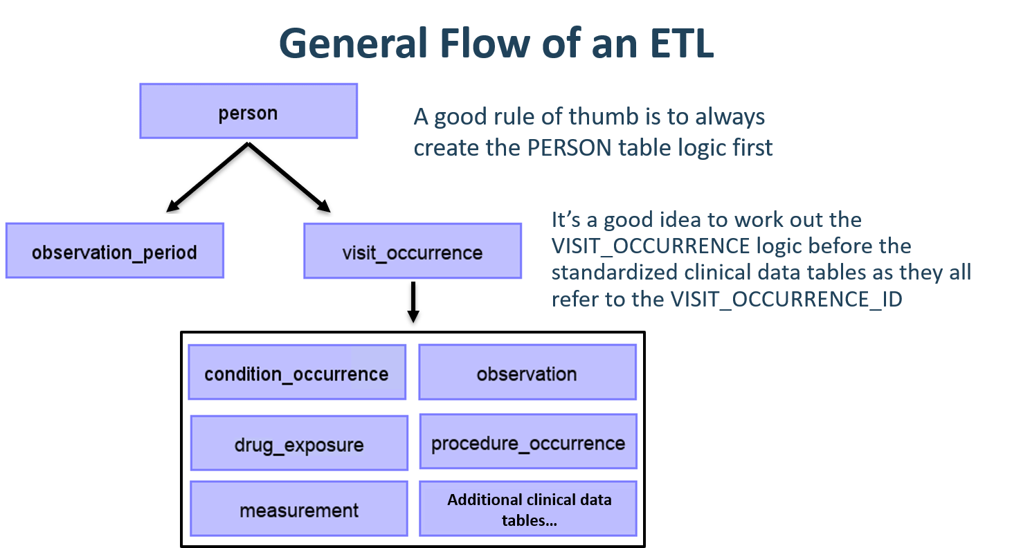
Figure 6.5: General flow of an ETL and which tables to map first.
It is often the case that, during CDM conversion, you will need to make provisions for intermediate tables. This could be for assigning the correct VISIT_OCCURRENCE_IDs to events, or for mapping source codes to standard concepts (doing this step on the fly is often very slow). Intermediate tables are 100% allowed and encouraged. What is discouraged is the persistence and reliance on these intermediate tables once the conversion is complete.
Mapping Example: Person Table
The Synthea data structure contains 20 columns in the patients table but not all were needed to populate the PERSON table, as seen in Figure 6.6. This is very common and should not be cause for alarm. In this example many of the data points in the Synthea patients table that were not used in the CDM PERSON table were additional identifiers like patient name, driver’s license number, and passport number.
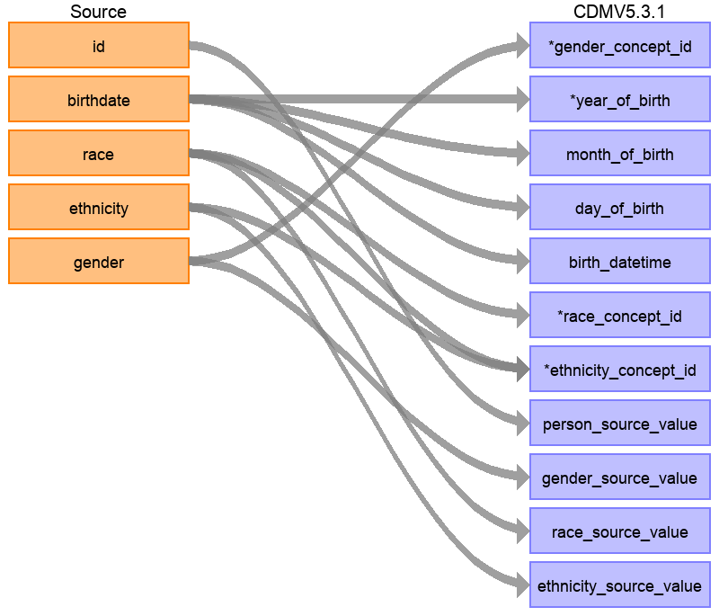
Figure 6.6: Mapping of Synthea Patients table to CDM PERSON table.
Table 6.1 below shows the logic that was imposed on the Synthea patients table to convert it to the CDM PERSON table. The ‘Destination Field’ discusses where in the CDM data is being mapped to. The ‘Source field’ highlights the column from the source table (in this case patients) that will be used to populate the CDM column. Finally, the ‘Logic & comments’ column gives explanations for the logic.
| Destination Field | Source field | Logic & comments |
|---|---|---|
| PERSON_ID | Autogenerate. The PERSON_ID will be generated at the time of implementation. This is because the id value from the source is a varchar value while the PERSON_ID is an integer. The id field from the source is set as the PERSON_SOURCE_VALUE to preserve that value and allow for error-checking if necessary. | |
| GENDER_CONCEPT_ID | gender | When gender = ‘M’ then set GENDER_CONCEPT_ID to 8507, when gender = ‘F’ then set to 8532. Drop any rows with missing/unknown gender. These two concepts were chosen as they are the only two standard concepts in the gender domain. The choice to drop patients with unknown genders tends to be site-based, though it is recommended they are removed as people without a gender are excluded from analyses. |
| YEAR_OF_BIRTH | birthdate | Take year from birthdate |
| MONTH_OF_BIRTH | birthdate | Take month from birthdate |
| DAY_OF_BIRTH | birthdate | Take day from birthdate |
| BIRTH_DATETIME | birthdate | With midnight as time 00:00:00. Here, the source did not supply a time of birth so the choice was made to set it at midnight. |
| RACE_CONCEPT_ID | race | When race = ‘WHITE’ then set as 8527, when race = ‘BLACK’ then set as 8516, when race = ‘ASIAN’ then set as 8515, otherwise set as 0. These concepts were chosen because they are the standard concepts belonging to the race domain that most closely align with the race categories in the source. |
| ETHNICITY_ CONCEPT_ID | race ethnicity | When race = ‘HISPANIC’, or when ethnicity in (‘CENTRAL_AMERICAN’, ‘DOMINICAN’, ‘MEXICAN’, ‘PUERTO_RICAN’, ‘SOUTH_AMERICAN’) then set as 38003563, otherwise set as 0. This is a good example of how multiple source columns can contribute to one CDM column. In the CDM ethnicity is represented as either Hispanic or not Hispanic so values from both the source column race and source column ethnicity will determine this value. |
| LOCATION_ID | ||
| PROVIDER_ID | ||
| CARE_SITE_ID | ||
| PERSON_SOURCE_ VALUE | id | |
| GENDER_SOURCE_ VALUE | gender | |
| GENDER_SOURCE_ CONCEPT_ID | ||
| RACE_SOURCE_ VALUE | race | |
| RACE_SOURCE_ CONCEPT_ID | ||
| ETHNICITY_ SOURCE_VALUE | ethnicity | In this case the ETHNICITY_SOURCE_VALUE will have more granularity than the ETHNICITY_CONCEPT_ID. |
| ETHNICITY_ SOURCE_CONCEPT_ID |
For more examples on how the Synthea dataset was mapped to the CDM please see the full specification document.32
6.3 Step 2: Create the Code Mappings
More and more source codes are being added to the OMOP Vocabulary all the time. This means that the coding systems in the data being transformed to the CDM may already be included and mapped. Check the VOCABULARY table in the OMOP Vocabulary to see which vocabularies are included. To extract the mapping from non-standard source codes (e.g. ICD-10CM codes) to standard concepts (e.g. SNOMED codes), we can use the records in the CONCEPT_RELATIONSHIP table having relationship_id = “Maps to”. For example, to find the standard concept ID for the ICD-10CM code ‘I21’ (“Acute Myocardial Infarction”), we can use the following SQL:
SELECT concept_id_2 standard_concept_id
FROM concept_relationship
INNER JOIN concept source_concept
  ON concept_id = concept_id_1
WHERE concept_code = 'I21'
  AND vocabulary_id = 'ICD10CM'
AND relationship_id = 'Maps to';| STANDARD_CONCEPT_ID |
|---|
| 312327 |
Unfortunately, sometimes the source data uses coding systems that are not in the Vocabulary. In this case, a mapping must be created from the source coding system to the Standard Concepts. Code mapping can be a daunting task, especially when there are many codes in the source coding system. There are several things that can be done to make the task easier:
- Focus on the most frequently used codes. A code that is never used or infrequently used is not worth the effort of mapping, since it will never be used in a real study.
- Make use of existing information whenever possible. For example, many national drug coding systems have been mapped to ATC. Although ATC is not detailed enough for many purposes, the concept relationships between ATC and RxNorm can be used to make good guesses of what the right RxNorm codes are.
- Use Usagi.
6.3.1 Usagi
Usagi is a tool to aid the manual process of creating a code mapping. It can make suggested mappings based on textual similarity of code descriptions. If the source codes are only available in a foreign language, we have found that Google Translate33 often gives surprisingly good translation of the terms into English. Usagi allows the user to search for the appropriate target concepts if the automated suggestion is not correct. Finally, the user can indicate which mappings are approved to be used in the ETL. Usagi is available on GitHub.34
Scope and Purpose
Source codes that need mapping are loaded into the Usagi (if the codes are not in English additional translations columns are needed). A term similarity approach is used to connect source codes to Vocabulary concepts. However, these code connections need to be manually reviewed and Usagi provides an interface to facilitate that. Usagi will only propose concepts that are marked as Standard concepts in the Vocabulary.
Process Overview
The typical sequence for using this software is:
- Load codes from your sources system (“source codes”) that you would like to map to Vocabulary concepts.
- Usagi will run a term similarity approach to map source codes to Vocabulary concepts.
- Leverage Usagi interface to check, and where needed, improve suggested mappings. Preferably an individual who has experience with the coding system and medical terminology should be used for this review.
- Export mapping to the Vocabulary’s SOURCE_TO_CONCEPT_MAP.
Importing Source Codes into Usagi
Export source codes from source system into a CSV or Excel (.xlsx) file. This should at least have columns containing the source code and an English source code description, however additional information about codes can be brought over as well (e.g. dose unit, or the description in the original language if translated). In addition to information about the source codes, the frequency of the code should preferably also be brought over, since this can help prioritize which codes should receive the most effort in mapping (e.g. you can have 1,000 source codes but only 100 are truly used within the system). If any source code information needs translating to English, use Google Translate.
Note: source code extracts should be broken out by domain (i.e. drugs, procedures, conditions, observations) and not lumped into one large file.
Source codes are loaded into Usagi from the File –> Import codes menu. From here an “Import codes …” will display as seen in Figure 6.7. In this figure, the source code terms were in Dutch and were also translated into English. Usagi will leverage the English translations to map to the standard vocabulary.
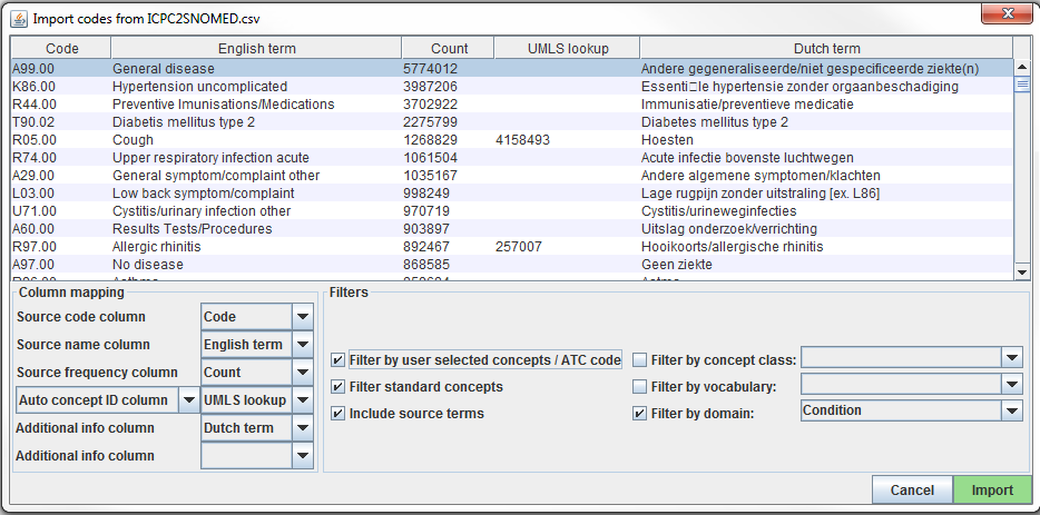
Figure 6.7: Usagi source code input screen.
The “Column mapping” section (bottom left) is where you define for Usagi how to use the imported table. If you mouse hover over the drop downs, a pop-up will appear defining each column. Usagi will not use the “Additional info” column(s) as information to associate source codes to Vocabulary concept codes; however, this additional information may help the individual reviewing the source code mapping and should be included.
Finally, in the “Filters” section (bottom right) you can set some restrictions for Usagi when mapping. For example, in Figure 6.7, the user is mapping the source codes only to concepts in the Condition domain. By default, Usagi only maps to Standard Concepts, but if the option “Filter standard concepts” is turned off, Usagi will also consider Classification Concepts. Hover your mouse over the different filters for additional information about the filter.
One special filter is “Filter by automatically selected concepts / ATC code”. If there is information that you can use to restrict the search, you can do so by providing a list of CONCEPT_IDs or an ATC code in the column indicated in the Auto concept ID column (semicolon-delimited). For example, in the case of drugs there might already be ATC codes assigned to each drug. Even though an ATC code does not uniquely identify a single RxNorm drug code, it does help limit the search space to only those concepts that fall under the ATC code in the Vocabulary. To use the ATC code, follow these steps:
- In the Column mapping section, switch from “Auto concept ID column” to “ATC column”
- In the Column mapping section, select the column containing the ATC code as “ATC column”.
- Turnon the “Filter by user selected concepts / ATC code” on in the Filters section.
You can also use other sources of information than the ATC code to restrict as well. In the example shown in the figure above, we used a partial mapping derived from UMLS to restrict the Usagi search. In that case we will need to use “Auto concept ID column”.
Once all your settings are finalized, click the “Import” button to import the file. The file import will take a few minutes as it is running the term similarity algorithm to map source codes.
Reviewing Source Code to Vocabulary Concept Maps
Once you have imported your input file of source codes, the mapping process begins. In Figure 6.8, you see the Usagi screen is made up of 3 main sections: an overview table, the selected mapping section, and place to perform searches. Note that in any of the tables, you can right-click to select the columns that are shown or hidden to reduce the visual complexity.

Figure 6.8: Usagi source code input screen.
Approving a Suggested Mapping
The “Overview Table” shows the current mapping of source codes to concepts. Right after importing source codes, this mapping contains the automatically generated suggested mappings based on term similarity and any search options. In the example in Figure 6.8, the English names of Dutch condition codes were mapped to standard concepts in the Condition domain, because the user restricted the search to that domain. Usagi compared the source code descriptions to concept names and synonyms to find the best match. Because the user had selected “Include source terms” Usagi also considered the names and synonyms of all source concepts in the vocabulary that map to a particular concept. If Usagi is unable to make a mapping, it will map to the CONCEPT_ID = 0.
It is suggested that someone with experience with coding systems help map source codes to their associated standard vocabulary. That individual will work through code by code in the “Overview Table” to either accept the mapping Usagi has suggested or choose a new mapping. For example in Figure 6.8 we see that the Dutch term “Hoesten” which was translated to the English term “Cough”. Usagi used “Cough” and mapped it to the Vocabulary concept of “4158493-C/O - cough”. There was a matching score of 0.58 associated to this matched pair (matching scores are typically 0 to 1 with 1 being a confident match), a score of 0.58 signifies that Usagi is not very sure of how well it has mapped this Dutch code to SNOMED. Let us say in this case, we are okay with this mapping, we can approve it by hitting the green “Approve” button in the bottom right hand portion of the screen.
Searching for a New Mapping
There will be cases where Usagi suggests a map and the user will be left to either try to find a better mapping or set the map to no concept (CONCEPT_ID = 0). In the example given in Figure 6.8, we see for the Dutch Term “Hoesten”, which was translated to “Cough”. Usagi’s suggestion was restricted by the concept identified in our automatically derived mapping from UMLS, and the result might not be optimal. In the Search Facility, we could search for other concepts using either the actual term itself or a search box query.
When using the manual search box, one should keep in mind that Usagi uses a fuzzy search, and does not support structured search queries, so for example not supporting Boolean operators like AND and OR.
To continue our example, suppose we used the search term “Cough” to see if we could find a better mapping. On the right of the Query section of the Search Facility, there is a Filters section, this provides options to trim down the results from the Vocabulary when searching for the search term. In this case we know we want to only find standard concepts, and we allow concepts to be found based on the names and synonyms of source concepts in the vocabulary that map to those standard concepts.
When we apply these search criteria we find “254761-Cough” and feel this may be an appropriate Vocabulary concept to map to our Dutch code. In order to do that we can hit the “Replace concept” button, which you will see in the “Selected Source Code” section update, followed by the “Approve” button. There is also an “Add concept” button, this allows for multiple standardized Vocabulary concepts to map to one source code (e.g. some source codes may bundle multiple diseases together while the standardized vocabulary may not).
Concept Information
When looking for appropriate concepts to map to, it is important to consider the “social life” of a concept. The meaning of a concept might depend partially on its place in the hierarchy, and sometimes there are “orphan concepts” in the vocabulary with few or no hierarchical relationships, which would be ill-suited as target concepts. Usagi will often report the number of parents and children a concept has, and it also possible to show more information by pressing ALT + C or selecting view –> Concept information in the top menu bar.
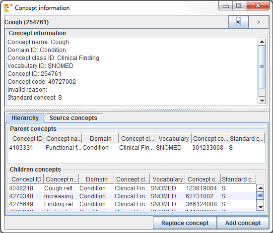
Figure 6.9: Usagi concept information panel.
Figure 6.9 shows the concept information panel. It shows general information about a concept, as well as its parents, children, and other source codes that map to the concept. Users can use this panel to navigate the hierarchy and potentially choose a different target concept.
Continue to move through this process, code by code, until all codes have been checked. In the list of source codes at the top of the screen, by selecting the column heading you can sort the codes. Often, we suggest going from the highest frequency codes to the lowest. In the bottom left of the screen you can see the number of codes that have approved mappings, and how many code occurrences that corresponds to.
It is possible to add comments to mappings, which could be used to document why a mapping decision was made.
Best Practices
- Use someone who has experience with coding schemes.
- By clicking on a column name, you can sort the columns in the “Overview Table”. It may be valuable to sort on “Match Score”; reviewing codes that Usagi is most confident on first may quickly knock out a significant chunk of codes. Also sorting on “Frequency” is valuable, spending more effort on frequent codes versus non-frequent is important.
- It is okay to map some codes to CONCEPT_ID = 0, some codes may not be worth it to find a good map and others may just lack a proper map.
- It is important to consider the context of a concept, specifically its parents and children.
Export the Usagi Map Created
Once you have created your map within USAGI, the best way to use it moving forward is to export it and append it to the Vocabulary SOURCE_TO_CONCEPT_MAP table.
To export your mappings, go to File –> Export source_to_concept_map. A pop-up will appear asking you which SOURCE_VOCABULARY_ID you would like to use, type in a short identifier. Usagi will use this identifier. as the SOURCE_VOCABULARY_ID which will allow you to identify your specific mapping in the SOURCE_TO_CONCEPT_MAP table.
After selecting the SOURCE_VOCABULARY_ID, you give your export CSV a name and save to location. The export CSV structure is in that of the SOURCE_TO_CONCEPT_MAP table. This mapping could be appended to the Vocabulary’s SOURCE_TO_CONCEPT_MAP table. It would also make sense to append a single row to the VOCABULARY table defining the SOURCE_VOCABULARY_ID you defined in the step above. Finally, it is important to note that only mappings with the “Approved” status will be exported into the CSV file; the mapping needs to be completed in USAGI in order to export it.
Updating an Usagi Mapping
Often a mapping is not a one-time effort. As data is updated perhaps new source codes are added, and the vocabulary is updated regularly, perhaps requiring an update of the mapping.
When the set of source codes is updated the following steps can support the update:
- Import the new source code file
- Choose File –> Apply previous mapping, and select the old Usagi mapping file
- Identify codes that haven’t inherited approved mappings from the old mapping, and map them as usual.
When the vocabulary is updated, follow these steps:
- Download the new vocabulary files from Athena
- Rebuild the Usagi index (Help –> Rebuild index)
- Open the mapping file
- Identify codes that map to concepts that in the new vocabulary version no longer are Standard concepts, and find more appropriate target concepts.
6.4 Step 3: Implement the ETL
Once the design and code mappings are completed, the ETL process can be implemented in a piece of software. When the ETL was being designed we recommended that people who are knowledgeable about the source and CDM work together on the task. Similarly, when the ETL is being implemented it is preferred to use people who have experience with working with data (particularly large data) and experience with implementing ETLs. This may mean working with individuals outside of your immediate group or hiring technical consultants to execute the implementation. It is also important to note that this is not a one-time expense. Moving forward it would be good to have someone or a team who spends at least some dedicated time to maintaining and running the ETL (this will become clearer in Section 6.7).
Implementation usually varies site to site and it largely depends on many factors including infrastructure, size of the database, the complexity of the ETL, and the technical expertise available. Because it depends on many factors the OHDSI community does not make a formal recommendation on how best to implement an ETL. There have been groups that use simple SQL builders, SAS, C#, Java, and Kettle. All have their advantages and disadvantages, and none are usable if there is nobody at the site who is familiar with the technology.
A few examples of different ETLs (listed in order of complexity):
- ETL-Synthea - A SQL builder written to convert the Synthea database
- ETL-CDMBuilder - A .NET application designed to transform multiple databases
- ETL-LambdaBuilder - A builder using the AWS lambda functionality
It should be noted that after several independent attempts, we have given up on developing the ‘ultimate’ user-friendly ETL tool. It is always the case that tools like that work well for 80% of the ETL, but for the remaining 20% of the ETL some low-level code needs to be written that is specific to a source database
Once the technical individuals are ready to start implementing, the ETL design document should be shared with them. There should be enough information in the documentation for them to get started however it should be expected that the developers have access to the ETL designers to ask questions during their development process. Logic that may be clear to the designers may be less clear to an implementer who might not be familiar with the data and CDM. The implementation phase should remain a team effort. It is considered acceptable practice to go through the process of CDM creation and testing between the implementers and designers, respectively, until both groups are in agreement that all logic has been executed correctly.
6.5 Step 4: Quality Control
For the extract, transform, load process, quality control is iterative. The typical pattern is to write logic -> implement logic -> test logic -> fix/write logic. There are many ways to go about testing a CDM but below are recommend steps that have been developed across the community through years of ETL implementation.
- Review of the ETL design document, computer code, and code mappings. Any one person can make mistakes, so always at least one other person should review what the what was done.
- The largest issues in the computer code tend to come from how the source codes in the native data are mapped to Standard Concepts. Mapping can get tricky, especially when it comes to date-specific codes like NDCs. Be sure to double check any area where mappings are done to ensure the correct source vocabularies are translated to the proper concept id.
- Manually compare all information on a sample of persons in the source and target data.
- It can be helpful to walk through one person’s data, ideally a person with a large number of unique records. Tracing through a single person can highlight issues if the data in the CDM is not how you expect it to look based on the agreed upon logic.
- Compare overall counts in the source and target data.
- There may be some expected differences in counts depending on how you chose to address certain issues. For instance, some collaborators choose to drop any people with a NULL gender since those people will not be included in analyses anyway. It may also be the case that visits in the CDM are constructed differently than visits or encounters in the native data. Therefore, when comparing overall counts between the source and CDM data be sure to account for and expect these differences.
- Replicate a study that has already been performed on the source data on the CDM version.
- This is a good way to understand any major differences between the source data and CDM version, though it is a little more time-intensive.
- Create unit tests meant to replicate a pattern in the source data that should be addressed in the ETL. For example, if your ETL specifies that patients without gender information should be dropped, create a unit test of a person without a gender and assess how the builder handles it.
- Unit testing is very handy when evaluating the quality and accuracy of an ETL conversion. It usually involves creating a much smaller dataset that mimics the structure of the source data you are converting. Each person or record in the dataset should test a specific piece of logic as written in the ETL document. Using this method, it is easy to trace back issues and to identify failing logic. The small size also enables the computer code to execute very quickly allowing for faster iterations and error identification.
These are high-level ways to approach quality control from an ETL standpoint. For more detail on the data quality efforts going on within OHDSI, please see Chapter 15.
6.6 ETL Conventions and THEMIS
As more groups converted data to the CDM it became apparent that conventions needed to be specified. For example, what should the ETL do in a situation where a person record lacks a birth year? The goal of the CDM is to standardized healthcare data however if every group handles data specific scenarios differently it makes it more difficult to systematically use data across the network.
The OHDSI community started documenting conventions to improve consistency across CDMs. These defined conventions, that the OHDSI community has agreed upon, can be found on the CDM Wiki.35 Each CDM table has its own set of conventions that can be referred to when designing an ETL. For example, persons are allowed to be missing a birth month or day, but if they lack a birth year the person should be dropped. In designing an ETL, refer to the conventions to help make certain design decisions that will be consistent with the community.
While it will never be possible to document all possible data scenarios that exist and what to do when they occur, there is an OHDSI work group trying to document common scenarios. THEMIS36 is made up of individuals in the community who gather conventions, clarify them, share them with the community for comment, and then document finalized conventions in the CDM Wiki. Themis is an ancient Greek Titaness of divine order, fairness, law, natural law, and custom which seemed a good fit for this groups remit. When performing an ETL, if there is a scenario that you are unsure how to handle, THEMIS recommends that a question about the scenario is posed on the OHDSI Forums.37 Most likely if you have a question, others in the community probably have it as well. THEMIS uses these discussions, as well as work group meetings and face-to-face discussions, to help inform what other conventions need to be documented.
6.7 CDM and ETL Maintenance
It is no small effort to design the ETL, create the mappings, implement the ETL, and build out quality control measures. Unfortunately, the effort does not stop there. There is a cycle of ETL maintenance that is a continuous process after the first CDM is built. Some common triggers that require maintenance are: changes in the source data, a bug in the ETL, a new OMOP Vocabulary is released, or the CDM itself has changed or updated. If one of these triggers occur the following might need updating: the ETL documentation, the software programming running the ETL, and test cases and quality controls.
Often a healthcare data source is forever changing. New data might be available (e.g. a new column in the data might exist). Patients’ scenarios that never existed before suddenly do (e.g. a new patient who has a death record before they were born). Your understanding of the data may improve (e.g. some of the records around inpatient child birth come across as outpatient due to how claims are processed). Not all changes in the source data may trigger a change in the ETL processing of it, however at a bare minimum the changes that break the ETL processing will need to be addressed.
If bugs are found, they should be addressed. However, it is important to keep in mind that not all bugs are created equal. For example, let’s say in the COST table the column cost was being rounded to a whole digit (e.g. the source data had $3.82 and this became $4.00 in the CDM). If the primary researchers using the data were mostly performing characterizations of patient’s drug exposures and conditions, a bug such as this is of little importance and can be addressed in the future. If the primary researchers using the data also included health economists, this would be a critical bug that need to be addressed immediately.
The OMOP Vocabulary is also ever changing just as our source data may be. In fact, the Vocabulary can have multiple releases in one given month as vocabularies update. Each CDM is run on a specific version of a Vocabulary and running on a newer improved Vocabulary could result in changes in how sources codes get mapped to in the standardized vocabularies. Often differences between Vocabularies are minor, so building a new CDM every time a new Vocabulary is released is not necessary. However, it is good practice to adopt a new Vocabulary once or twice a year which would require reprocessing the CDM again. It is rare that changes in a new version of a Vocabulary would require the ETL code itself to be updated.
The final trigger that could require CDM or ETL maintenance is when the common data model itself updates. As the community grows and new data requirements are found this may lead to additional data being stored in the CDM. This might mean data that you previously were not storing in the CDM might have a location in a new CDM version. Less frequently are changes to existing CDM structure, however it is a possibility. For example, the CDM has adopted DATETIME fields over the original DATE fields which could cause an error in ETL processing. CDM versions are not released often and sites can choose when they migrate.
6.8 Final Thoughts on ETL
The ETL process is diff for many reasons, not the least of which is the fact that we are all processing unique source data, making it hard to create a “one-size-fits-all” solution. However, over the years we have learned the following hard-won lessons.
- The 80/20 rule. If you can avoid it do not spend too much time manually mapping source codes to concepts sets. Ideally, map the source codes that cover the majority of your data. This should be enough to get you started and you can address any remaining codes in the future based on use cases.
- It’s ok if you lose data that is not of research quality. Often these are the records that would be discarded before starting an analysis anyway, we just remove them during the ETL process instead.
- A CDM requires maintenance. Just because you complete an ETL does not mean you do not need to touch it ever again. Your raw data might change, there might be a bug in the code, there may be new vocabulary or an update to the CDM. Plan to allocate resources for these changes so your ETL is always up-to-date.
- For support starting the OHDSI CDM, performing your database conversion, or running the analytics tools, please visit our Implementers Forum.38
6.9 Summary
There is a generally agreed upon process for how to approach an ETL, including
- Data experts and CDM experts together design the ETL
- People with medical knowledge create the code mappings
- A technical person implements the ETL
- All are involved in quality control
Tools have been developed by the OHDSI community to facilitate these steps and are freely available for use
There are many ETL examples and agreed upon conventions you can use as a guide
6.10 Exercises
Exercise 6.1 Put the steps of the ETL process in the proper order:
- Data experts and CDM experts together design the ETL
- A technical person implements the ETL
- People with medical knowledge create the code mappings
- All are involved in quality control
Exercise 6.2 Using OHDSI resources of your choice, spot four issues with the PERSON record show in Table 6.2 (table abbreviated for space):
| Column | Value |
|---|---|
| PERSON_ID | A123B456 |
| GENDER_CONCEPT_ID | 8532 |
| YEAR_OF_BIRTH | NULL |
| MONTH_OF_BIRTH | NULL |
| DAY_OF_BIRTH | NULL |
| RACE_CONCEPT_ID | 0 |
| ETHNICITY_CONCEPT_ID | 8527 |
| PERSON_SOURCE_VALUE | A123B456 |
| GENDER_SOURCE_VALUE | F |
| RACE_SOURCE_VALUE | WHITE |
| ETHNICITY_SOURCE_VALUE | NONE PROVIDED |
Exercise 6.3 Let us try to generate VISIT_OCCURRENCE records. Here is some example logic written for Synthea: Sort data in ascending order by PATIENT, START, END. Then by PERSON_ID, collapse lines of claim as long as the time between the END of one line and the START of the next is <=1 day. Each consolidated inpatient claim is then considered as one inpatient visit, set:
- MIN(START) as VISIT_START_DATE
- MAX(END) as VISIT_END_DATE
- “IP” as PLACE_OF_SERVICE_SOURCE_VALUE
If you see a set of visits as shown in Figure 6.10 in your source data, how would you expect the resulting VISIT_OCCURRENCE record(s) to look in the CDM?
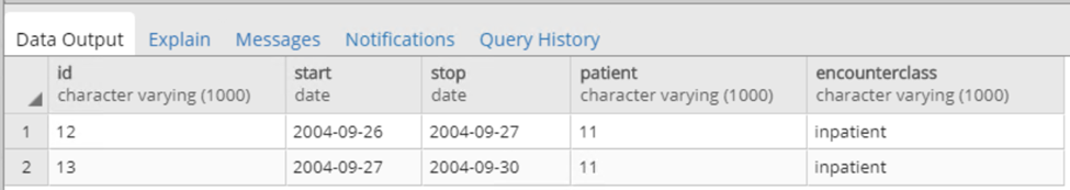
Figure 6.10: Example source data.
Suggested answers can be found in Appendix E.3.
SyntheaTM is a patient generator that aims to model real patients. Data are created based on parameters passed to the application.The structure of the data can be found here: https://github.com/synthetichealth/synthea/wiki.↩︎