Chapter 18 Method Validity

Chapter lead: Martijn Schuemie

When considering method validity we aim to answer the question

Is this method valid for answering this question?

“Method” includes not only the study design, but also the data and the implementation of the design. Method validity is therefore somewhat of a catch-all; it is often not possible to observe good method validity without good data quality, clinical validity, and software validity. Those aspects of evidence quality should have already been addressed separately before we consider method validity.

The core activity when establishing method validity is evaluating whether important assumptions in the analysis have been met. For example, we assume that propensity-score matching makes two populations comparable, but we need to evaluate whether this is the case. Where possible, empirical tests should be performed to verify these assumptions. We can for example generate diagnostics to show that our two populations are indeed comparable on a wide range of characteristics after matching. In OHDSI we have developed many standardized diagnostics that should be generated and evaluated whenever an analysis is performed.

In this chapter we will focus on the validity of methods use in population-level estimation. We will first briefly highlight some study design-specific diagnostics, and will then discuss diagnostics that are applicable to most if not all population-level estimation studies. Following this is a step-by-step description of how to execute these diagnostics using the OHDSI tools. We close this chapter with an advanced topic, reviewing the OHDSI Methods Benchmark and its application to the OHDSI Methods Library.

18.1 Design-Specific Diagnostics

For each study design there are diagnostics specific to such a design. Many of these diagnostics are implemented and readily available in the R packages of the OHDSI Methods Library. For example, Section 12.9 lists a wide range of diagnostics generated by the CohortMethod package, including:

Propensity score distribution to asses initial comparability of cohorts.
Propensity model to identify potential variables that should be excluded from the model.
Covariate balance to evaluate whether propensity score adjustment has made the cohorts comparable (as measured through baseline covariates).
Attrition to observe how many subjects were excluded in the various analysis steps, which may inform on the generalizability of the results to the initial cohorts of interest.
Power to assess whether enough data is available to answer the question.
Kaplan Meier curve to asses typical time to onset, and whether the proportionality assumption underlying Cox models is met.

Other study designs require different diagnostics to test the different assumptions in those designs. For example, for the self-controlled case series (SCCS) design we may check the necessary assumption that the end of observation is independent of the outcome. This assumption is often violated in the case of serious, potentially lethal, events such as myocardial infarction. We can evaluate whether the assumption holds by generating the plot shown in Figure 18.1, which shows histograms of the time to observation period end for those that are censored, and those that are uncensored. In our data we consider those whose observation period ends at the end date of data capture (the date when observation stopped for the entire data base, for example the date of extraction, or the study end date) to be uncensored, and all others to be censored. In Figure 18.1 we see only minor differences between the two distributions, suggesting our assumptions holds.

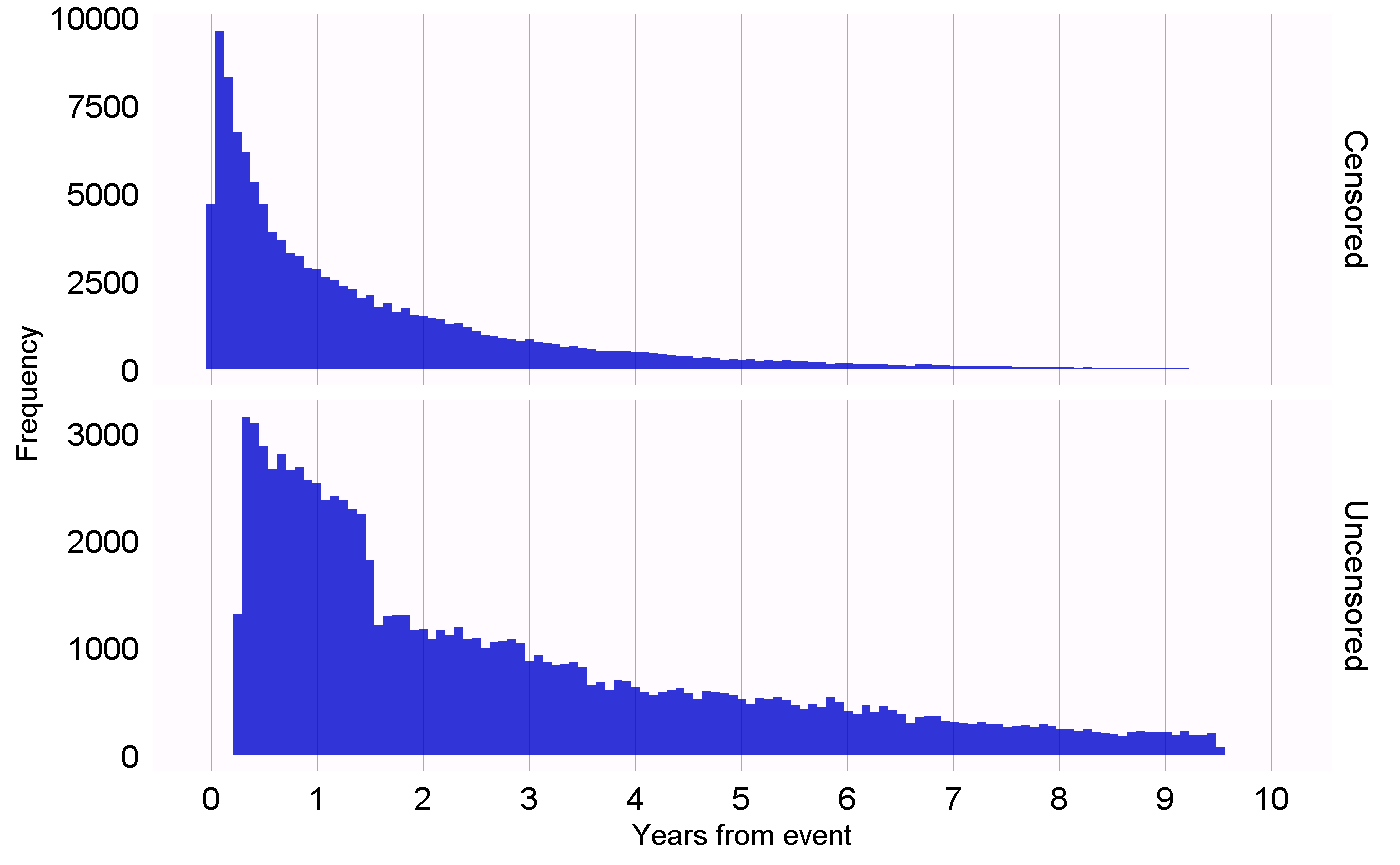
Figure 18.1: Time to observation end for those that are censored, and those that are uncensored.

18.2 Diagnostics for All Estimation

Next to the design-specific diagnostics, there are also several diagnostics that are applicable across all causal effect estimation methods. Many of these rely on the use of control hypotheses, research questions where the answer is already known. Using control hypotheses we can then evaluate whether our design produces results in line with the truth. Controls can be divided into negative controls and positive controls.

18.2.1 Negative Controls

Negative controls are exposure-outcome pairs where one believes no causal effect exists, and it includes negative controls or “falsification endpoints” (Prasad and Jena 2013) that have been recommended as a means to detect confounding, (Lipsitch, Tchetgen Tchetgen, and Cohen 2010) selection bias, and measurement error. (Arnold et al. 2016) For example, in one study (Zaadstra et al. 2008) investigating the relationship between childhood diseases and later multiple sclerosis (MS), the authors include three negative controls that are not believed to cause MS: a broken arm, concussion, and tonsillectomy. Two of these three controls produce statistically significant associations with MS, suggesting that the study may be biased.

We should select negative controls that are comparable to our hypothesis of interest, which means we typically select exposure-outcome pairs that either have the same exposure as the hypothesis of interest (so-called “outcome controls”) or the same outcome (“exposure controls”). Our negative controls should further meet these criteria:

The exposure should not cause the outcome. One way to think of causation is to think of the counterfactual: could the outcome be caused (or prevented) if a patient was not exposed, compared to if the patient had been exposed? Sometimes this is clear, for example ACEi are known to cause angioedema. Other times this is far less obvious. For example, a drug that may cause hypertension can therefore indirectly cause cardiovascular diseases that are a consequence of the hypertension.
The exposure should also not prevent or treat the outcome. This is just another causal relationship that should be absent if we are to believe the true effect size (e.g. the hazard ratio) is 1.
The negative control should exist in the data, ideally with sufficient numbers. We try to achieve this by prioritizing candidate negative controls based on prevalence.
Negative controls should ideally be independent. For example, we should avoid having negative controls that are either ancestors of each other (e.g. “ingrown nail” and “ingrown nail of foot”) or siblings (e.g. “fracture of left femur” and “fracture of right femur”).
Negative controls should ideally have some potential for bias. For example, the last digit of someone’s social security number is basically a random number, and is unlikely to show confounding. It should therefore not be used as a negative control.

Some argue that negative controls should also have the same confounding structure as the exposure-outcome pair of interest. (Lipsitch, Tchetgen Tchetgen, and Cohen 2010) However, we believe this confounding structure is unknowable; the relationships between variables found in reality is often far more complex than people imagine. Also, even if the confounder structure was known, it is unlikely that a negative control exists having that exact same confounding structure, but lacking the direct causal effect. For this reason in OHDSI we rely on a large number of negative controls, assuming that such a set represents many different types of bias, including the ones present in the hypothesis of interest.

The absence of a causal relationship between an exposure and an outcome is rarely documented. Instead, we often make the assumption that a lack of evidence of a relationship implies the lack of a relationship. This assumption is more likely to hold if the exposure and outcome have both been studied extensively, so a relationship could have been detected. For example, the lack of evidence for a completely novel drug likely implies a lack of knowledge, not the lack of a relationship. With this principle in mind we have developed a semi-automated procedure for selecting negative controls. (Voss et al. 2016) In brief, information from literature, product labels, and spontaneous reporting is automatically extracted and synthesized to produce a candidate list of negative controls. This list must then undergo manual review, not only to verify that the automated extraction was accurate, but also to impose additional criteria such as biological plausibility.

18.2.2 Positive Controls

To understand the behavior of a method when the true relative risk is smaller or greater than one requires the use of positive controls where the null is believed to not be true. Unfortunately, real positive controls for observational research tend to be problematic for three reasons. First, in most research contexts, for example when comparing the effect of two treatments, there is a paucity of positive controls relevant for that specific context. Second, even if positive controls are available, the magnitude of the effect size may not be known with great accuracy, and often depends on the population in which one measures it. Third, when treatments are widely known to cause a particular outcome, this shapes the behavior of physicians prescribing the treatment, for example by taking actions to mitigate the risk of unwanted outcomes, thereby rendering the positive controls useless as a means for evaluation. (Noren et al. 2014)

In OHDSI we therefore use synthetic positive controls, (Schuemie, Hripcsak, et al. 2018) created by modifying a negative control through injection of additional, simulated occurrences of the outcome during the time at risk of the exposure. For example, assume that, during exposure to ACEi, n occurrences of our negative control outcome “ingrowing nail” were observed. If we now add an additional n simulated occurrences during exposure, we have doubled the risk. Since this was a negative control, the relative risk compared to the counterfactual was one, but after injection, it becomes two.

One issue that stands important is the preservation of confounding. The negative controls may show strong confounding, but if we inject additional outcomes randomly, these new outcomes will not be confounded, and we may therefore be optimistic in our evaluation of our capacity to deal with confounding for positive controls. To preserve confounding, we want the new outcomes to show similar associations with baseline subject-specific covariates as the original outcomes. To achieve this, for each outcome we train a model to predict the survival rate with respect to the outcome during exposure using covariates captured prior to exposure. These covariates include demographics, as well as all recorded diagnoses, drug exposures, measurements, and medical procedures. An L1-regularized Poisson regression (Suchard et al. 2013) using 10-fold cross-validation to select the regularization hyperparameter fits the prediction model. We then use the predicted rates to sample simulated outcomes during exposure to increase the true effect size to the desired magnitude. The resulting positive control thus contains both real and simulated outcomes.

Figure 18.2 depicts this process. Note that although this procedure simulates several important sources of bias, it does not capture all. For example, some effects of measurement error are not present. The synthetic positive controls imply constant positive predictive value and sensitivity, which may not be true in reality.

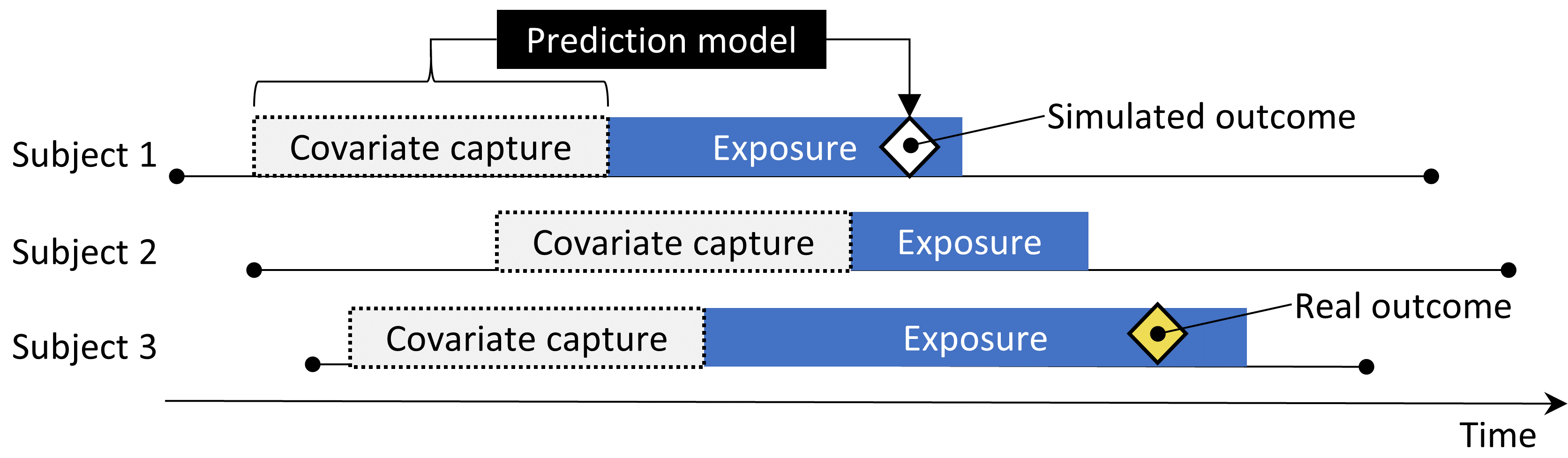
Figure 18.2: Synthesizing positive controls from negative controls.

Although we refer to a single true “effect size” for each control, different methods estimate different statistics of the treatment effect. For negative controls, where we believe no causal effect exists, all such statistics, including the relative risk, hazard ratio, odds ratio, incidence rate ratio, both conditional and marginal, as well as the average treatment effect in the treated (ATT) and the overall average treatment effect (ATE) will be identical to 1. Our process for creating positive controls synthesizes outcomes with a constant incidence rate ratio over time and between patients, using a model conditioned on the patient where this ratio is held constant, up to the point where the marginal effect is achieved. The true effect size is thus guaranteed to hold as the marginal incidence rate ratio in the treated. Under the assumption that our outcome model used during synthesis is correct, this also holds for the conditional effect size and the ATE. Since all outcomes are rare, odds ratios are all but identical to the relative risk.

18.2.3 Empirical Evaluation

Based on the estimates of a particular method for the negative and positive controls, we can then understand the operating characteristics by computing a range of metrics, for example:

Area Under the receiver operator Curve (AUC): the ability to discriminate between positive and negative controls.
Coverage: how often the true effect size is within the 95% confidence interval.
Mean precision: precision is computed as $1/(standard\ error)^2$, higher precision means narrower confidence intervals. We use the geometric mean to account for the skewed distribution of the precision.
Mean squared error (MSE): Mean squared error between the log of the effect size point-estimate and the log of the true effect size.
Type 1 error: For negative controls, how often was the null rejected (at $\alpha = 0.05$). This is equivalent to the false positive rate and $1 - specificity$.
Type 2 error: For positive controls, how often was the null not rejected (at $\alpha = 0.05$). This is equivalent to the false negative rate and $1 - sensitivity$.
Non-estimable: For how many of the controls was the method unable to produce an estimate? There can be various reasons why an estimate cannot be produced, for example because there were no subjects left after propensity score matching, or because no subjects remained having the outcome.

Depending on our use case, we can evaluate whether these operating characteristics are suitable for our goal. For example, if we wish to perform signal detection, we may care about type 1 and type 2 error, or if we are willing to modify our $\alpha$ threshold, we may inspect the AUC instead.

18.2.4 P-Value Calibration

Often the type 1 error (at $\alpha = 0.05$) is larger than 5%. In other words, we are often more likely than 5% to reject the null hypothesis when in fact the null hypothesis is true. The reason is that the p-value only reflects random error, the error due to having a limited sample size. It does not reflect systematic error, for example the error due to confounding. OHDSI has developed a process for calibrating p-values to restore the type 1 error to nominal. (Schuemie et al. 2014) We derive an empirical null distribution from the actual effect estimates for the negative controls. These negative control estimates give us an indication of what can be expected when the null hypothesis is true, and we use them to estimate an empirical null distribution.

Formally, we fit a Gaussian probability distribution to the estimates, taking into account the sampling error of each estimate. Let $\hat{\theta}_i$ denote the estimated log effect estimate (relative risk, odds or incidence rate ratio) from the $i$th negative control drug–outcome pair, and let $\hat{\tau}_i$ denote the corresponding estimated standard error, $i=1,\ldots,n$. Let $\theta_i$ denote the true log effect size (assumed 0 for negative controls), and let $\beta_i$ denote the true (but unknown) bias associated with pair $i$ , that is, the difference between the log of the true effect size and the log of the estimate that the study would have returned for control $i$ had it been infinitely large. As in the standard p-value computation, we assume that $\hat{\theta}_i$ is normally distributed with mean $\theta_i + \beta_i$ and standard deviation $\hat{\tau}_i^2$. Note that in traditional p-value calculation, $\beta_i$ is always assumed to be equal to zero, but that we assume the $\beta_i$’s, arise from a normal distribution with mean $\mu$ and variance $\sigma^2$. This represents the null (bias) distribution. We estimate $\mu$ and $\sigma^2$ via maximum likelihood. In summary, we assume the following:

\[\beta_i \sim N(\mu,\sigma^2) \text{ and } \hat{\theta}_i \sim N(\theta_i + \beta_i, \tau_i^2)\]

where $N(a,b)$ denotes a Gaussian distribution with mean $a$ and variance $b$, and estimate $\mu$ and $\sigma^2$ by maximizing the following likelihood:

\[L(\mu, \sigma | \theta, \tau) \propto \prod_{i=1}^{n}\int p(\hat{\theta}_i|\beta_i, \theta_i, \hat{\tau}_i)p(\beta_i|\mu, \sigma) \text{d}\beta_i\]

yielding maximum likelihood estimates $\hat{\mu}$ and $\hat{\sigma}$. We compute a calibrated p-value that uses the empirical null distribution. Let $\hat{\theta}_{n+1}$ denote the log of the effect estimate from a new drug–outcome pair, and let $\hat{\tau}_{n+1}$ denote the corresponding estimated standard error. From the aforementioned assumptions and assuming $\beta_{n+1}$ arises from the same null distribution, we have the following:

\[\hat{\theta}_{n+1} \sim N(\hat{\mu}, \hat{\sigma} + \hat{\tau}_{n+1})\]

When $\hat{\theta}_{n+1}$ is smaller than $\hat{\mu}$, the one-sided calibrated p-value for the new pair is then

\[\phi\left(\frac{\theta_{n+1} - \hat{\mu}}{\sqrt{\hat{\sigma}^2 + \hat{\tau}_{n+1}^2}}\right)\]

where $\phi(\cdot)$ denotes the cumulative distribution function of the standard normal distribution. When $\hat{\theta}_{n+1}$ is bigger than $\hat{\mu}$, the one-sided calibrated p-value is then

\[1-\phi\left(\frac{\theta_{n+1} - \hat{\mu}}{\sqrt{\hat{\sigma}^2 + \hat{\tau}_{n+1}^2}}\right)\]

18.2.5 Confidence Interval Calibration

Similarly, we typically observe that the coverage of the 95% confidence interval is less than 95%: the true effect size is inside the 95% confidence interval less than 95% of the time. For confidence interval calibration (Schuemie, Hripcsak, et al. 2018) we extend the framework for p-value calibration by also making use of our positive controls. Typically, but not necessarily, the calibrated confidence interval is wider than the nominal confidence interval, reflecting the problems unaccounted for in the standard procedure (such as unmeasured confounding, selection bias and measurement error) but accounted for in the calibration.

Formally, we assume that $beta_i$, the bias associated with pair $i$, again comes from a Gaussian distribution, but this time using a mean and standard deviation that are linearly related to $theta_i$, the true effect size:

\[\beta_i \sim N(\mu(\theta_i) , \sigma^2(\theta_i))\]

where

\[\mu(\theta_i) = a + b \times \theta_i \text{ and } \\ \sigma(\theta_i) ^2= c + d \times \mid \theta_i \mid\]

We estimate $a$, $b$, $c$ and $d$ by maximizing the marginalized likelihood in which we integrate out the unobserved $\beta_i$:

\[l(a,b,c,d | \theta, \hat{\theta}, \hat{\tau} ) \propto \prod_{i=1}^{n}\int p(\hat{\theta}_i|\beta_i, \theta_i, \hat{\tau}_i)p(\beta_i|a,b,c,d,\theta_i) \text{d}\beta_i ,\]

yielding maximum likelihood estimates $(\hat{a}, \hat{b}, \hat{c}, \hat{d})$.

We compute a calibrated CI that uses the systematic error model. Let $\hat{\theta}_{n+1}$ again denote the log of the effect estimate for a new outcome of interest, and let $\hat{\tau}_{n+1}$ denote the corresponding estimated standard error. From the assumptions above, and assuming $\beta_{n+1}$ arises from the same systematic error model, we have:

\[\hat{\theta}_{n+1} \sim N( \theta_{n+1} + \hat{a} + \hat{b} \times \theta_{n+1}, \hat{c} + \hat{d} \times \mid \theta_{n+1} \mid + \hat{\tau}_{n+1}^2) .\]

We find the lower bound of the calibrated 95% CI by solving this equation for $\theta_{n+1}$:

\[\Phi\left( \frac{\theta_{n+1} + \hat{a} + \hat{b} \times \theta_{n+1}-\hat{\theta}_{n+1}} {\sqrt{(\hat{c} + \hat{d} \times \mid \theta_{n+1} \mid) + \hat{\tau}_{n+1}^2}} \right) = 0.025 ,\]

where $\Phi(\cdot)$ denotes the cumulative distribution function of the standard normal distribution. We find the upper bound similarly for probability 0.975. We define the calibrated point estimate by using probability 0.5.

Both p-value calibration and confidence interval calibration are implemented in the EmpiricalCalibration package.

18.2.6 Replication Across Sites

Another form of method validation comes from executing the study across several different databases that represent different populations, different health care systems, and/or different data capture processes. Prior research has shown that executing the same study design across different databases can produce vastly different effect size estimates, (Madigan et al. 2013) suggesting that either the effect differs greatly for different populations, or that the design does not adequately address the different biases found in the different databases. In fact, we observe that accounting for residual bias in a database through empirical calibration of confidence intervals can greatly reduce between-study heterogeneity. (Schuemie, Hripcsak, et al. 2018)

One way to express between-database heterogeneity is the $I^2$ score, describing the percentage of total variation across studies that is due to heterogeneity rather than chance. (Higgins et al. 2003) A naive categorization of values for $I^2$ would not be appropriate for all circumstances, although one could tentatively assign adjectives of low, moderate, and high to $I^2$ values of 25%, 50%, and 75%. In a study estimating the effects for many depression treatments using a new-user cohort design with large-scale propensity score adjustment, (Schuemie, Ryan, et al. 2018) observed only 58% of the estimates to have an $I^2$ below 25%. After empirical calibration this increased to 83%.

Observing between-database heterogeneity casts doubt on the validity of the estimates. Unfortunately, the inverse is not true. Not observing heterogeneity does not guarantee an unbiased estimate. It is not unlikely that all databases share a similar bias, and that all estimates are therefore consistently wrong.

18.2.7 Sensitivity Analyses

When designing a study there are often design choices that are uncertain. For example, should propensity score matching of stratification be used? If stratification is used, how many strata? What is the appropriate time-at-risk? When faced with such uncertainty, one solution is to evaluate various options, and observe the sensitivity of the results to the design choice. If the estimate remains the same under various options, we can say the study is robust to the uncertainty.

This definition of sensitivity analysis should not be confused with the definitions used by others such as, Rosenbaum (2005) who defines sensitivity analysis to “appraise how the conclusions of a study might be altered by hidden biases of various magnitudes.”

18.3 Method Validation in Practice

Here we build on the example in Chapter 12, where we investigate the effect of ACE inhibitors (ACEi) on the risk of angioedema and acute myocardial infarction (AMI), compared to thiazides and thiazide-like diuretics (THZ). In that chapter we already explore many of the diagnostics specific to the design we used, the cohort method. Here, we apply additional diagnostics that could also have been applied had other designs been used. If the study is implemented using ATLAS as described in Section 12.7 these diagnostics are available in the Shiny app that is included in the study R package generated by ATLAS. If the study is implemented using R instead, as described in Section 12.8, then R functions available in the various packages should be used, as described in the next sections.

18.3.1 Selecting Negative Controls

We must select negative controls, exposure-outcome pairs where no causal effect is believed to exist. For comparative effect estimation such as our example study, we select negative control outcomes that are believed to be neither caused by the target nor the comparator exposure. We want enough negative controls to make sure we have a diverse mix of biases represented in the controls, and also to allow empirical calibration. As a rule-of-thumb we typically aim to have 50-100 such negative controls. We could come up with these controls completely manually, but fortunately ATLAS provides features to aid the selection of negative controls using data from literature, product labels, and spontaneous reports.

To generate a candidate list of negative controls, we first must create a concept set containing all exposures of interest. In this case we select all ingredients in the ACEi and THZ classes, as shown in Figure 18.3.

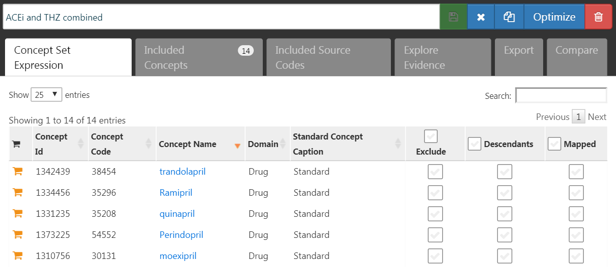
Figure 18.3: A concept set containing the concepts defining the target and comparator exposures.

Next, we go to the “Explore Evidence” tab, and click on the button. Generating the evidence overview will take a few minutes, after which you can click on the button. This will open the list of outcomes as shown in Figure 18.4.

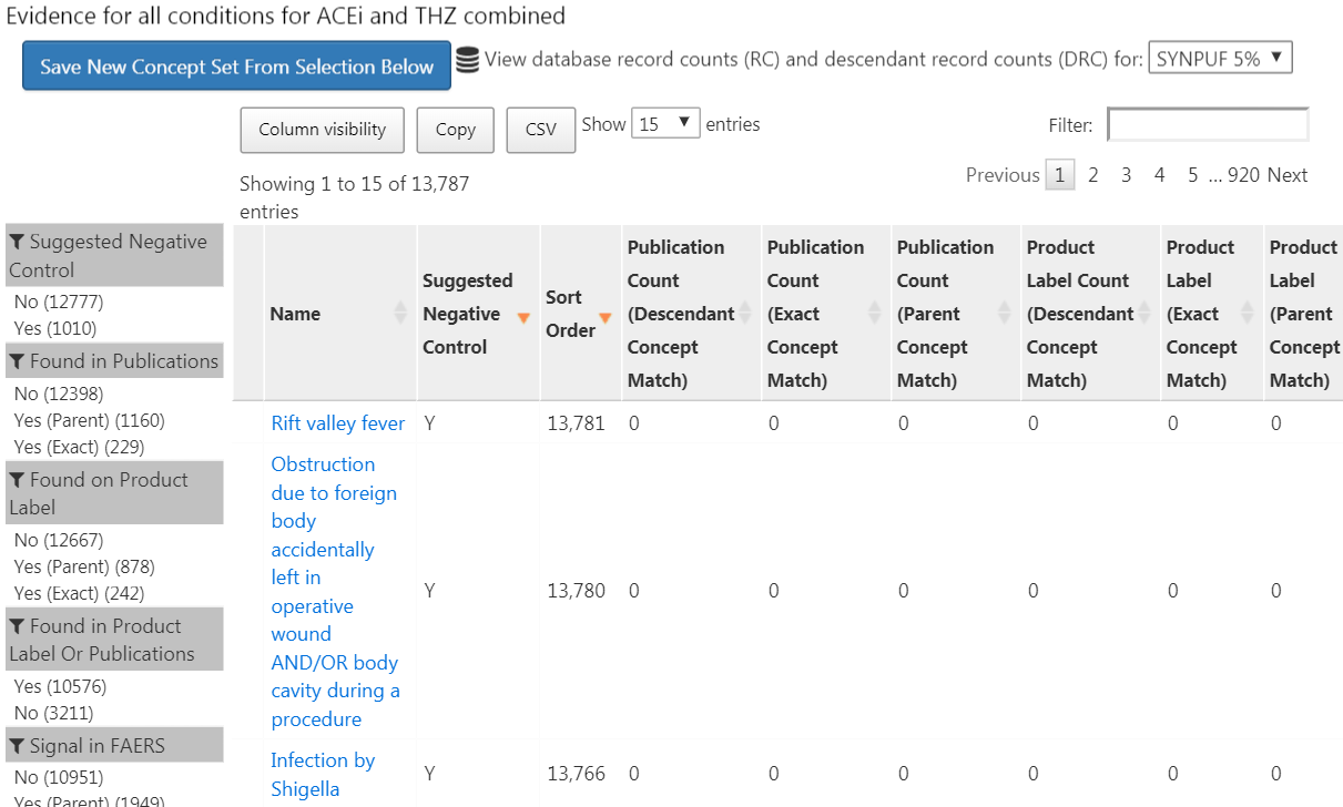
Figure 18.4: Candidate control outcomes with an overview of the evidence found in literature, product labels, and spontaneous reports.

This list shows condition concepts, along with an overview of the evidence linking the condition to any of the exposures we defined. For example, we see the number of publications that link the exposures to the outcomes found in PubMed using various strategies, the number of product labels of our exposures of interest that list the condition as a possible adverse effect, and the number of spontaneous reports. By default the list is sorted to show candidate negative controls first. It is then sorted by the “Sort Order,” which represents the prevalence of the condition in a collection of observational databases. The higher the Sort Order, the higher the prevalence. Although the prevalence in these databases might not correspond with the prevalence in the database we wish to run the study, it is likely a good approximation.

The next step is to manually review the candidate list, typically starting at the top, so with the most prevalent condition, and working our way down until we are satisfied we have enough. One typical way to do this is to export the list to a CSV (comma separated values) file, and have clinicians review these, considering the criteria mentioned in Section 18.2.1.

For our example study we select the 76 negative controls listed in Appendix C.1.

18.3.2 Including Controls

Once we have defined our set of negative controls we must include them in our study. First we must define some logic for turning our negative control condition concepts into outcome cohorts. Section 12.7.3 discusses how ATLAS allows creating such cohorts based on a few choices the user must make. Often we simply choose to create a cohort based on any occurrence of a negative control concept or any of its descendants. If the study is implemented in R, then SQL (Structured Query Language) can be used to construct the negative control cohorts. Chapter 9 describes how cohorts can be created using SQL and R. We leave it as an exercise for the reader to write the appropriate SQL and R.

The OHDSI tools also provide functionality for automatically generating and including positive controls derived from the negative controls. This functionality can be found in the Evaluation Settings section in ATLAS described in Section 12.7.3, and it is implemented in the synthesizePositiveControls function in the MethodEvaluation package. Here we generate three positive controls for each negative control, with true effect sizes of 1.5, 2, and 4, using a survival model:

library(MethodEvaluation)
# Create a data frame with all negative control exposure-
# outcome pairs, using only the target exposure (ACEi = 1).
eoPairs <- data.frame(exposureId = 1,
                      outcomeId = ncs)

pcs <- synthesizePositiveControls(
  connectionDetails = connectionDetails,
  cdmDatabaseSchema = cdmDbSchema,
  exposureDatabaseSchema = cohortDbSchema,
  exposureTable = cohortTable,
  outcomeDatabaseSchema = cohortDbSchema,
  outcomeTable = cohortTable,
  outputDatabaseSchema = cohortDbSchema,
  outputTable = cohortTable,
  createOutputTable = FALSE,
  modelType = "survival",
  firstExposureOnly = TRUE,
  firstOutcomeOnly = TRUE,
  removePeopleWithPriorOutcomes = TRUE,
  washoutPeriod = 365,
  riskWindowStart = 1,
  riskWindowEnd = 0,
  endAnchor = "cohort end",
  exposureOutcomePairs = eoPairs,
  effectSizes = c(1.5, 2, 4),
  cdmVersion = cdmVersion,
  workFolder = file.path(outputFolder, "pcSynthesis"))

Note that we must mimic the time-at-risk settings used in our estimation study design. The synthesizePositiveControls function will extract information about the exposures and negative control outcomes, fit outcome models per exposure-outcome pair, and synthesize outcomes. The positive control outcome cohorts will be added to the cohort table specified by cohortDbSchema and cohortTable. The resulting pcs data frame contains the information on the synthesized positive controls.

Next we must execute the same study used to estimate the effect of interest to also estimate effects for the negative and positive controls. Setting the set of negative controls in the comparisons dialog in ATLAS instructs ATLAS to compute estimates for these controls. Similarly, specifying that positive controls be generated in the Evaluation Settings includes these in our analysis. In R, the negative and positive controls should be treated as any other outcome. All estimation packages in the OHDSI Methods Library readily allow estimation of many effects in an efficient manner.

18.3.3 Empirical Performance

Figure 18.5 shows the estimated effect sizes for the negative and positive controls included in our example study, stratified by true effect size. This plot is included in the Shiny app that comes with the study R package generated by ATLAS, and can be generated using the plotControls function in the MethodEvaluation package. Note that the number of controls is often lower than what was defined because there was not enough data to either produce an estimate or to synthesize a positive control.

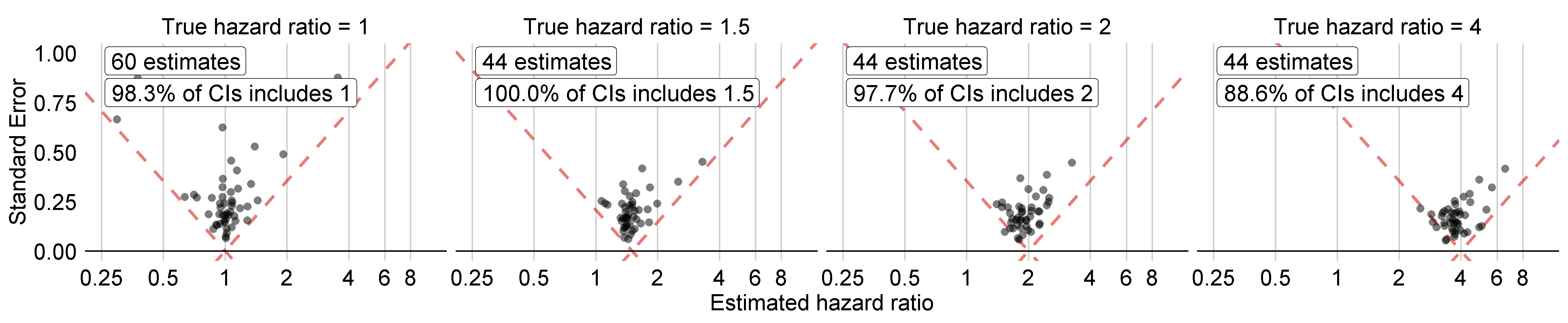
Estimates for the negative (true hazard ratio = 1) and positive controls (true hazard ratio > 1). Each dot represents a control. Estimates below the dashed line have a confidence interval that doesn't include the true effect size.

Figure 18.5: Estimates for the negative (true hazard ratio = 1) and positive controls (true hazard ratio > 1). Each dot represents a control. Estimates below the dashed line have a confidence interval that doesn’t include the true effect size.

Based on these estimates we can compute the metrics shown in Table 18.1 using the computeMetrics function in the MethodEvaluation package.

Table 18.1: Method performance metrics derived from the negative and positive control estimates.
Metric	Value
AUC	0.96
Coverage	0.97
Mean Precision	19.33
MSE	2.08
Type 1 error	0.00
Type 2 error	0.18
Non-estimable	0.08

We see that coverage and type 1 error are very close to their nominal values of 95% and 5%, respectively, and that the AUC is very high. This is certainly not always the case.

Note that although in Figure 18.5 not all confidence intervals include one when the true hazard ratio is one, the type 1 error in Table 18.1 is 0%. This is an exceptional situation, caused by the fact that confidence intervals in the Cyclops package are estimated using likelihood profiling, which is more accurate than traditional methods but can result in asymmetric confidence intervals. The p-value instead is computed assuming symmetrical confidence intervals, and this is what was used to compute the type 1 error.

18.3.4 P-Value Calibration

We can use the estimates for our negative controls to calibrate our p-values. This is done automatically in the Shiny app, and can be done manually in R. Assuming we have created the summary object summ as described in Section 12.8.6, we can plot the empirical calibration effect plot:

# Estimates for negative controls (ncs) and outcomes of interest (ois):
ncEstimates <- summ[summ$outcomeId %in% ncs, ]
oiEstimates <- summ[summ$outcomeId %in% ois, ]

library(EmpiricalCalibration)
plotCalibrationEffect(logRrNegatives = ncEstimates$logRr,
                      seLogRrNegatives = ncEstimates$seLogRr,
                      logRrPositives = oiEstimates$logRr,
                      seLogRrPositives = oiEstimates$seLogRr,
                      showCis = TRUE)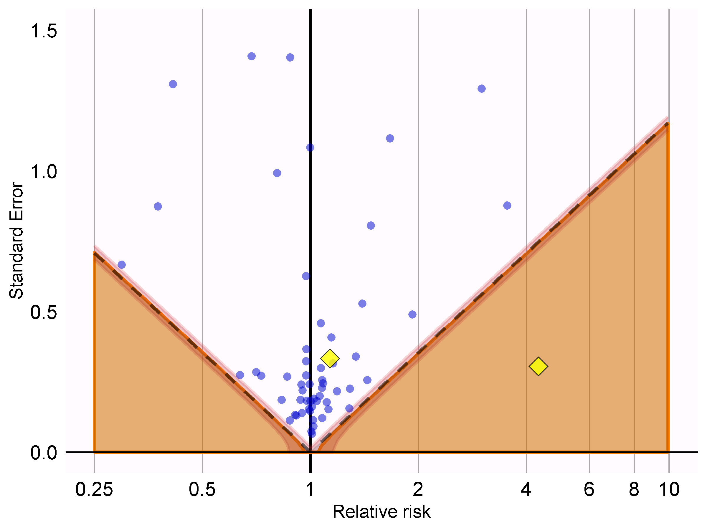

$P-value calibration: estimates below the dashed line have a conventional p < 0.05. Estimates in the shaded area have calibrated p < 0.05. The narrow band around the edge of the shaded area denotes the 95\% credible interval. Dots indicate negative controls. Diamonds indicate outcomes of interest.$

Figure 18.6: P-value calibration: estimates below the dashed line have a conventional p < 0.05. Estimates in the shaded area have calibrated p < 0.05. The narrow band around the edge of the shaded area denotes the 95% credible interval. Dots indicate negative controls. Diamonds indicate outcomes of interest.

In Figure 18.6 we see that the shaded area almost exactly overlaps with the area denoted by the dashed lines, indicating hardly any bias was observed for the negative controls. One of the outcomes of interest (AMI) is above the dashed line and the shaded area, indicating we cannot reject the null according to both the uncalibrated and calibrated p-value. The other outcome (angioedema) clearly stands out from the negative control, and falls well within the area where both uncalibrated and calibrated p-values are smaller than 0.05.

We can compute the calibrated p-values:

null <- fitNull(logRr = ncEstimates$logRr,
                seLogRr = ncEstimates$seLogRr)
calibrateP(null,
           logRr= oiEstimates$logRr,
           seLogRr = oiEstimates$seLogRr)

## [1] 1.604351e-06 7.159506e-01

And contrast these with the uncalibrated p-values:

oiEstimates$p

## [1] [1] 1.483652e-06 7.052822e-01

As expected, because little to no bias was observed, the uncalibrated and calibrated p-values are very similar.

18.3.5 Confidence Interval Calibration

Similarly, we can use the estimates for our negative and positive controls to calibrate the confidence intervals. The Shiny app automatically reports the calibrate confidence intervals. In R we can calibrate intervals using the fitSystematicErrorModel and calibrateConfidenceInterval functions in the EmpiricalCalibration package, as described in detail in the “Empirical calibration of confidence intervals” vignette.

Before calibration, the estimated hazard ratios (95% confidence interval) are 4.32 (2.45 - 8.08) and 1.13 (0.59 - 2.18), for angioedema and AMI respectively. The calibrated hazard ratios are 4.75 (2.52 - 9.04) and 1.15 (0.58 - 2.30).

18.3.6 Between-Database Heterogeneity

Just as we executed our analysis on one database, in this case the IBM MarketScan Medicaid (MDCD) database, we can also run the same analysis code on other databases that adhere to the Common Data Model (CDM). Figure 18.7 shows the forest plot and meta-analytic estimates (assuming random effects) (DerSimonian and Laird 1986) across a total of five databases for the outcome of angioedema. This figure was generated using the plotMetaAnalysisForest function in the EvidenceSynthesis package.

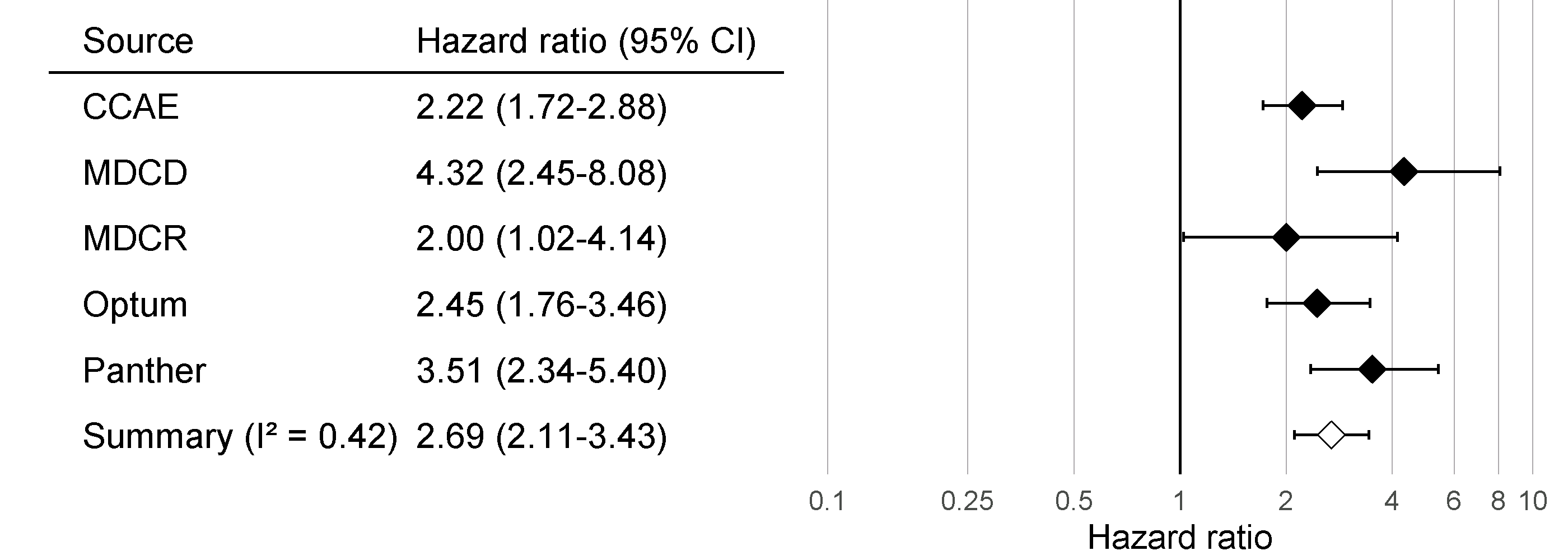
$Effect size estimates and 95\% confidence intervals (CI) from five different databases and a meta-analytic estimate when comparing ACE inhibitors to thiazides and thiazide-like diuretics for the risk of angioedema.$

Figure 18.7: Effect size estimates and 95% confidence intervals (CI) from five different databases and a meta-analytic estimate when comparing ACE inhibitors to thiazides and thiazide-like diuretics for the risk of angioedema.

Although all confidence intervals are above one, suggesting agreement on the fact that there is an effect, the $I^2$ suggests between-database heterogeneity. However, if we compute the $I^2$ using the calibrated confidence intervals as shown in Figure 18.8, we see that this heterogeneity can be explained by the bias measured in each database through the negative and positive controls. The empirical calibration appears to properly take this bias into account.

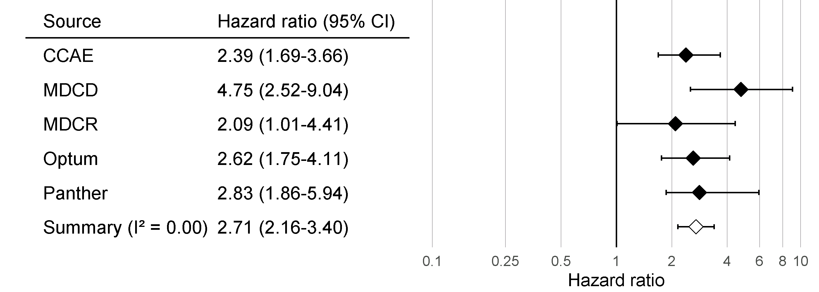
$Calibrated Effect size estimates and 95\% confidence intervals (CI) from five different databases and a meta-analytic estimate for the hazard ratio of angioedema when comparing ACE inhibitors to thiazides and thiazide-like diuretics.$

Figure 18.8: Calibrated Effect size estimates and 95% confidence intervals (CI) from five different databases and a meta-analytic estimate for the hazard ratio of angioedema when comparing ACE inhibitors to thiazides and thiazide-like diuretics.

18.3.7 Sensitivity Analyses

One of the design choices in our analysis was to use variable-ratio matching on the propensity score. However, we could have also used stratification on the propensity score. Because we are uncertain about this choice, we may decide to use both. Table 18.2 shows the effect size estimates for AMI and angioedema, both calibrated and uncalibrated, when using variable-ratio matching and stratification (with 10 equally-sized strata).

Table 18.2: Uncalibrated and calibrated hazard ratios (95% confidence interval) for the two analysis variants.
Outcome	Adjustment	Uncalibrated	Calibrated
Angioedema	Matching	4.32 (2.45 - 8.08)	4.75 (2.52 - 9.04)
Angioedema	Stratification	4.57 (3.00 - 7.19)	4.52 (2.85 - 7.19)
Acute myocardial infarction	Matching	1.13 (0.59 - 2.18)	1.15 (0.58 - 2.30)
Acute myocardial infarction	Stratification	1.43 (1.02 - 2.06)	1.45 (1.03 - 2.06)

We see that the estimates from the matched and stratified analysis are in strong agreement, with the confidence intervals for stratification falling completely inside of the confidence intervals for matching. This suggests that our uncertainty around this design choice does not impact the validity of our estimates. Stratification does appear to give us more power (narrower confidence intervals), which is not surprising since matching results in loss of data, whereas stratification does not. The price for this could be an increase in bias, due to within-strata residual confounding, although we see no evidence of increased bias reflected in the calibrated confidence intervals.

Study diagnostics allow us to evaluate design choices even before fully executing a study. It is recommended not to finalize the protocol before generating and reviewing all study diagnostics. To avoid p-hacking (adjusting the design to achieve a desired result), this should be done while blinded to the effect size estimate of interest.

18.4 OHDSI Methods Benchmark

Although the recommended practice is to empirically evaluate a method’s performance within the context that it is applied, using negative and positive controls that are in ways similar to the exposures-outcomes pairs of interest (for example using the same exposure or the same outcome) and on the database used in the study, there is also value in evaluating a method’s performance in general. This is why the OHDSI Methods Evaluation Benchmark was developed. The benchmark evaluates performance using a wide range of control questions, including those with chronic or acute outcomes, and long-term or short-term exposures. The results on this benchmark can help demonstrate the overall usefulness of a method, and can be used to form a prior belief about the performance of a method when a context-specific empirical evaluation is not (yet) available. The benchmark consists of 200 carefully selected negative controls that can be stratified into eight categories, with the controls in each category either sharing the same exposure or the same outcome. From these 200 negative controls, 600 synthetic positive controls are derived as described in Section 18.2.2. To evaluate a method, it must be used to produce effect size estimates for all controls, after which the metrics described in Section 18.2.3 can be computed. The benchmark is publicly available, and can be deployed as described in the Running the OHDSI Methods Benchmark vignette in the MethodEvaluation package.

We have run all the methods in the OHDSI Methods Library through this benchmark, with various analysis choices per method. For example, the cohort method was evaluated using propensity score matching, stratification, and weighting. This experiment was executed on four large observational healthcare databases. The results, viewable in an online Shiny app⁶³, show that although several methods show high AUC (the ability to distinguish positive controls from negative controls), most methods in most settings demonstrate high type 1 error and low coverage of the 95% confidence interval, as shown in Figure 18.9.

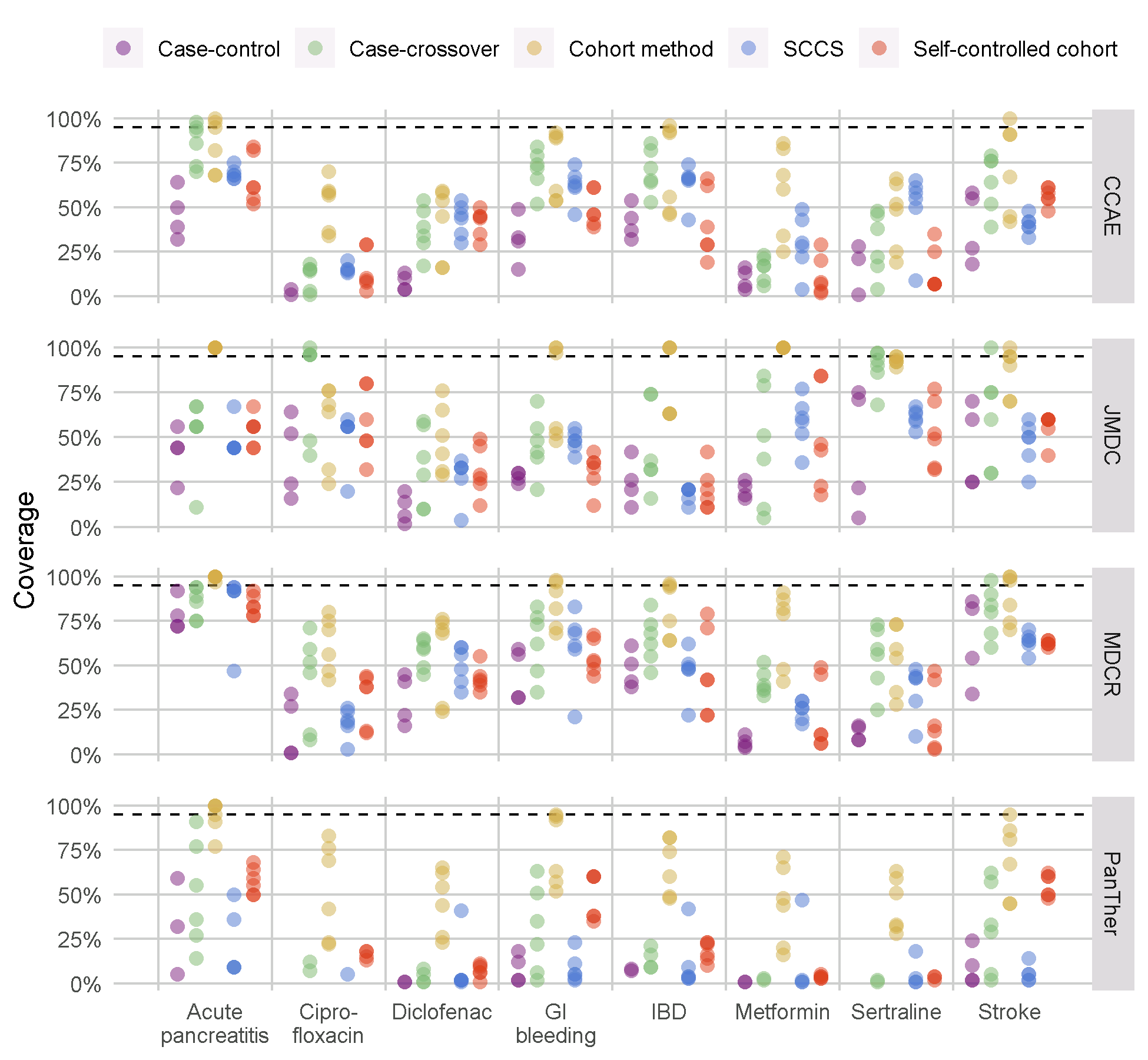
$Coverage of the 95\% confidence interval for the methods in the Methods Library. Each dot represents the performance of a specific set of analysis choices. The dashed line indicates nominal performance (95\% coverage). SCCS = Self-Controlled Case Series, GI = Gastrointestinal, IBD = inflammatory bowel disease.$

Figure 18.9: Coverage of the 95% confidence interval for the methods in the Methods Library. Each dot represents the performance of a specific set of analysis choices. The dashed line indicates nominal performance (95% coverage). SCCS = Self-Controlled Case Series, GI = Gastrointestinal, IBD = inflammatory bowel disease.

This emphasizes the need for empirical evaluation and calibration: if no empirical evaluation is performed, which is true for almost all published observational studies, we must assume a prior informed by the results in Figure 18.9, and conclude that it is likely that the true effect size is not contained in the 95% confidence interval!

Our evaluation of the designs in the Methods Library also shows that empirical calibration restores type 1 error and coverage to their nominal values, although often at the cost of increasing type 2 error and decreasing precision.

18.5 Summary

A method’s validity depends on whether the assumptions underlying the method are met.
Where possible, these assumptions should be empirically tested using study diagnostics.
Control hypotheses, questions where the answer is known, should be used to evaluate whether a specific study design produces answers in line with the truth.
Often, p-values and confidence intervals do not demonstrate nominal characteristics as measured using control hypotheses.
These characteristics can often be restored to nominal using empirical calibration.
Study diagnostics can be used to guide analytic design choices and adapt the protocol, as long as the researcher remains blinded to the effect of interest to avoid p-hacking.

References

Arnold, B. F., A. Ercumen, J. Benjamin-Chung, and J. M. Colford. 2016. “Brief Report: Negative Controls to Detect Selection Bias and Measurement Bias in Epidemiologic Studies.” Epidemiology 27 (5): 637–41.

DerSimonian, R., and N. Laird. 1986. “Meta-analysis in clinical trials.” Control Clin Trials 7 (3): 177–88.

Higgins, J. P., S. G. Thompson, J. J. Deeks, and D. G. Altman. 2003. “Measuring inconsistency in meta-analyses.” BMJ 327 (7414): 557–60.

Lipsitch, M., E. Tchetgen Tchetgen, and T. Cohen. 2010. “Negative controls: a tool for detecting confounding and bias in observational studies.” Epidemiology 21 (3): 383–88.

Madigan, D., P. B. Ryan, M. Schuemie, P. E. Stang, J. M. Overhage, A. G. Hartzema, M. A. Suchard, W. DuMouchel, and J. A. Berlin. 2013. “Evaluating the impact of database heterogeneity on observational study results.” Am. J. Epidemiol. 178 (4): 645–51.

Noren, G. N., O. Caster, K. Juhlin, and M. Lindquist. 2014. “Zoo or savannah? Choice of training ground for evidence-based pharmacovigilance.” Drug Saf 37 (9): 655–59.

Prasad, V., and A. B. Jena. 2013. “Prespecified falsification end points: can they validate true observational associations?” JAMA 309 (3): 241–42.

Rosenbaum, P. 2005. “Sensitivity Analysis in Observational Studies.” In Encyclopedia of Statistics in Behavioral Science. American Cancer Society. https://doi.org/10.1002/0470013192.bsa606.

Schuemie, M. 2018. “Empirical confidence interval calibration for population-level effect estimation studies in observational healthcare data.” Proc. Natl. Acad. Sci. U.S.A. 115 (11): 2571–7.

Schuemie, M. J., P. B. Ryan, W. DuMouchel, M. A. Suchard, and D. Madigan. 2014. “Interpreting observational studies: why empirical calibration is needed to correct p-values.” Stat Med 33 (2): 209–18.

Schuemie, M. J., P. B. Ryan, G. Hripcsak, D. Madigan, and M. A. Suchard. 2018. “Improving reproducibility by using high-throughput observational studies with empirical calibration.” Philos Trans A Math Phys Eng Sci 376 (2128).

Suchard, M. A., S. E. Simpson, Ivan Zorych, P. B. Ryan, and David Madigan. 2013. “Massive Parallelization of Serial Inference Algorithms for a Complex Generalized Linear Model.” ACM Trans. Model. Comput. Simul. 23 (1): 10:1–10:17. https://doi.org/10.1145/2414416.2414791.

Voss, E. A., R. D. Boyce, P. B. Ryan, J. van der Lei, P. R. Rijnbeek, and M. J. Schuemie. 2016. “Accuracy of an Automated Knowledge Base for Identifying Drug Adverse Reactions.” J Biomed Inform, December.

Zaadstra, B. M., A. M. Chorus, S. van Buuren, H. Kalsbeek, and J. M. van Noort. 2008. “Selective association of multiple sclerosis with infectious mononucleosis.” Mult. Scler. 14 (3): 307–13.

http://data.ohdsi.org/MethodEvalViewer/↩︎