Chapter 12 Population-Level Estimation
Chapter leads: Martijn Schuemie, David Madigan, Marc Suchard & Patrick Ryan
Observational healthcare data, such as administrative claims and electronic health records, offer opportunities to generate real-world evidence about the effect of treatments that can meaningfully improve the lives of patients. In this chapter we focus on population-level effect estimation, which refers to the estimation of average causal effects of exposures (e.g. medical interventions such as drug exposures or procedures) on specific health outcomes of interest. In what follows, we consider two different estimation tasks:
- Direct effect estimation: estimating the effect of an exposure on the risk of an outcome, as compared to no exposure.
- Comparative effect estimation: estimating the effect of an exposure (the target exposure) on the risk of an outcome, as compared to another exposure (the comparator exposure).
In both cases, the patient-level causal effect contrasts a factual outcome, i.e., what happened to the exposed patient, with a counterfactual outcome, i.e., what would have happened had the exposure not occurred (direct) or had a different exposure occurred (comparative). Since any one patient reveals only the factual outcome (the fundamental problem of causal inference), the various effect estimation designs employ different analytic devices to shed light on the counterfactual outcomes.
Use-cases for population-level effect estimation include treatment selection, safety surveillance, and comparative effectiveness. Methods can test specific hypotheses one at a time (e.g. ‘signal evaluation’) or explore multiple-hypotheses-at-once (e.g. ‘signal detection’). In all cases, the objective remains the same: to produce a high-quality estimate of the causal effect.
In this chapter we first describe various population-level estimation study designs, all of which are implemented as R packages in the OHDSI Methods Library. We then detail the design of an example estimation study, followed by step-by-step guides of how to implement the design using ATLAS and R. Finally, we review the various outputs generated by the study, including study diagnostics and effect size estimates.
12.1 The Cohort Method Design
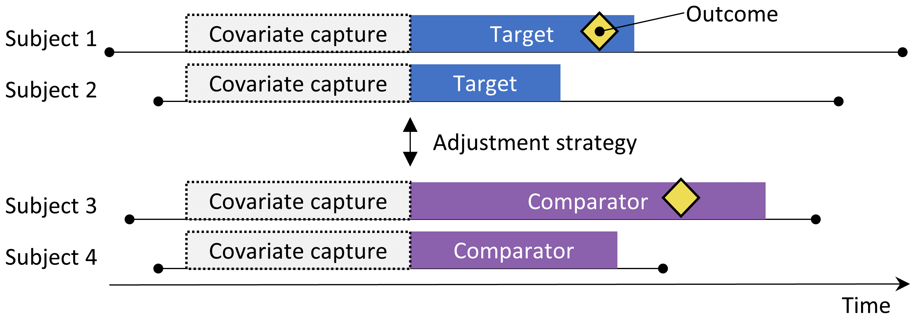
Figure 12.1: The new-user cohort design. Subjects observed to initiate the target treatment are compared to those initiating the comparator treatment. To adjust for differences between the two treatment groups several adjustment strategies can be used, such as stratification, matching, or weighting by the propensity score, or by adding baseline characteristics to the outcome model. The characteristics included in the propensity model or outcome model are captured prior to treatment initiation.
The cohort method attempts to emulate a randomized clinical trial. (Hernan and Robins 2016) Subjects that are observed to initiate one treatment (the target) are compared to subjects initiating another treatment (the comparator) and are followed for a specific amount of time following treatment initiation, for example the time they stay on the treatment. We can specify the questions we wish to answer in a cohort study by making the five choices highlighted in Table 12.1.
| Choice | Description |
|---|---|
| Target cohort | A cohort representing the target treatment |
| Comparator cohort | A cohort representing the comparator treatment |
| Outcome cohort | A cohort representing the outcome of interest |
| Time-at-risk | At what time (often relative to the target and comparator cohort start and end dates) do we consider the risk of the outcome? |
| Model | The model used to estimate the effect while adjusting for differences between the target and comparator |
The choice of model specifies, among others, the type of outcome model. For example, we could use a logistic regression, which evaluates whether or not the outcome has occurred, and produces an odds ratio. A logistic regression assumes the time-at-risk is of the same length for both target and comparator, or is irrelevant. Alternatively, we could choose a Poisson regression which estimates the incidence rate ratio, assuming a constant incidence rate. Often a Cox regression is used which considers time to first outcome to estimate the hazard ratio, assuming proportional hazards between target and comparator.
A key concern is that the patients receiving the target treatment may systematically differ from those receiving the comparator treatment. For example, suppose the target cohort is on average 60 years old, whereas the comparator cohort is on average 40 years old. Comparing target to comparator with respect to any age-related health outcome (e.g. stroke) might then show substantial differences between the cohorts. An uninformed investigator might reach the conclusion there is a causal association between the target treatment and stroke as compared to the comparator. More prosaically or commonplace, the investigator might conclude that there exist target patients that experienced stroke that would not have done so had they received the comparator. This conclusion could well be entirely incorrect! Maybe those target patients disproportionately experienced stroke simply because they are older; maybe the target patients that experienced stroke might well have done so even if they had received the comparator. In this context, age is a “confounder.” One mechanism to deal with confounders in observational studies is through propensity scores.
12.1.1 Propensity Scores
In a randomized trial, a (virtual) coin toss assigns patients to their respective groups. Thus, by design, the probability that a patient receives the target treatment as against the comparator treatment does not relate in any way to patient characteristics such as age. The coin has no knowledge of the patient, and, what’s more, we know with certainty the exact probability that a patient receives the target exposure. As a consequence, and with increasing confidence as the number of patients in the trial increases, the two groups of patients essentially cannot differ systematically with respect to any patient characteristic. This guaranteed balance holds true for characteristics that the trial measured (such as age) as well as characteristics that the trial failed to measure, such as patient genetic factors.
For a given patient, the propensity score (PS) is the probability that that patient received the target treatment as against the comparator. (Rosenbaum and Rubin 1983) In a balanced two-arm randomized trial, the propensity score is 0.5 for every patient. In a propensity score-adjusted observational study, we estimate the probability of a patient receiving the target treatment based on what we can observe in the data on and before the time of treatment initiation (irrespective of the treatment they actually received). This is a straightforward predictive modeling application; we fit a model (e.g. a logistic regression) that predicts whether a subject receives the target treatment, and use this model to generate predicted probabilities (the PS) for each subject. Unlike in a standard randomized trial, different patients will have different probabilities of receiving the target treatment. The PS can be used in several ways including matching target subjects to comparator subjects with similar PS, stratifying the study population based on the PS, or weighting subjects using Inverse Probability of Treatment Weighting (IPTW) derived from the PS. When matching we can select just one comparator subject for each target subject, or we can allow more than one comparator subject per target subject, a technique know as variable-ratio matching. (Rassen et al. 2012)
For example, suppose we use one-on-one PS matching, and that Jan has a priori probability of 0.4 of receiving the target treatment and in fact receives the target treatment. If we can find a patient (named Jun) that also had an a priori probability of 0.4 of receiving the target treatment but in fact received the comparator, the comparison of Jan and Jun’s outcomes is like a mini-randomized trial, at least with respect to measured confounders. This comparison will yield an estimate of the Jan-Jun causal contrast that is as good as the one randomization would have produced. Estimation then proceeds as follows: for every patient that received the target, find one or more matched patients that received the comparator but had the same prior probability of receiving the target. Compare the outcome for the target patient with the outcomes for the comparator patients within each of these matched groups.
Propensity scoring controls for measured confounders. In fact, if treatment assignment is “strongly ignorable” given measured characteristics, propensity scoring will yield an unbiased estimate of the causal effect. “Strongly ignorable” essentially means that there are no unmeasured confounders, and that the measured confounders are adjusted for appropriately. Unfortunately this is not a testable assumption. See Chapter 18 for further discussion of this issue.
12.1.2 Variable Selection
In the past, PS were computed based on manually selected characteristics, and although the OHDSI tools can support such practices, we prefer using many generic characteristics (i.e. characteristics that are not selected based on the specific exposures and outcomes in the study). (Tian, Schuemie, and Suchard 2018) These characteristics include demographics, as well as all diagnoses, drug exposures, measurement, and medical procedures observed prior to and on the day of treatment initiation. A model typically involves 10,000 to 100,000 unique characteristics, which we fit using large-scale regularized regression (Suchard et al. 2013) implemented in the Cyclops package. In essence, we let the data decide which characteristics are predictive of the treatment assignment and should be included in the model.
Some have argued that a data-driven approach to covariate selection that does not depend on clinical expertise to specify the “right” causal structure runs the risk of erroneously including so-called instrumental variables and colliders, thus increasing variance and potentially introducing bias. (Hernan et al. 2002) However, these concerns are unlikely to have a large impact in real-world scenarios. (Schneeweiss 2018) Furthermore, in medicine the true causal structure is rarely known, and when different researchers are asked to identify the ‘right’ covariates to include for a specific research question, each researcher invariably comes up with a different list, thus making the process irreproducible. Most importantly, our diagnostics such as inspection of the propensity model, evaluating balance on all covariates, and including negative controls would identify most problems related to colliders and instrumental variables.
12.1.3 Caliper
Since propensity scores fall on a continuum from 0 to 1, exact matching is rarely possible. Instead, the matching process finds patients that match the propensity score of a target patient(s) within some tolerance known as a “caliper.” Following Austin (2011), we use a default caliper of 0.2 standard deviations on the logit scale.
12.1.4 Overlap: Preference Scores
The propensity method requires that matching patients exist! As such, a key diagnostic shows the distribution of the propensity scores in the two groups. To facilitate interpretation, the OHDSI tools plot a transformation of the propensity score called the “preference score”. (Walker et al. 2013) The preference score adjusts for the “market share” of the two treatments. For example, if 10% of patients receive the target treatment (and 90% receive the comparator treatment), then patients with a preference score of 0.5 have a 10% probability of receiving the target treatment. Mathematically, the preference score is
\[\ln\left(\frac{F}{1-F}\right)=\ln\left(\frac{S}{1-S}\right)-\ln\left(\frac{P}{1-P}\right)\]
Where \(F\) is the preference score, \(S\) is the propensity score, and \(P\) is the proportion of patients receiving the target treatment.
Walker et al. (2013) discuss the concept of “empirical equipoise.” They accept exposure pairs as emerging from empirical equipoise if at least half of the exposures are to patients with a preference score of between 0.3 and 0.7.
12.1.5 Balance
Good practice always checks that the PS adjustment succeeds in creating balanced groups of patients. Figure 12.19 shows the standard OHDSI output for checking balance. For each patient characteristic, this plots the standardized difference between means between the two exposure groups before and after PS adjustment. Some guidelines recommend an after-adjustment standardized difference upper bound of 0.1. (Rubin 2001)
12.2 The Self-Controlled Cohort Design
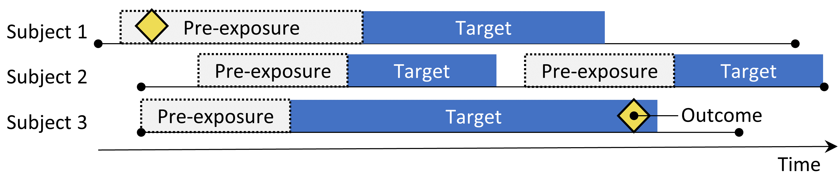
Figure 12.2: The self-controlled cohort design. The rate of outcomes during exposure to the target is compared to the rate of outcomes in the time pre-exposure.
The self-controlled cohort (SCC) design (Ryan, Schuemie, and Madigan 2013) compares the rate of outcomes during exposure to the rate of outcomes in the time just prior to the exposure. The four choices shown in Table 12.2 define a self-controlled cohort question.
| Choice | Description |
|---|---|
| Target cohort | A cohort representing the treatment |
| Outcome cohort | A cohort representing the outcome of interest |
| Time-at-risk | At what time (often relative to the target cohort start and end dates) do we consider the risk of the outcome? |
| Control time | The time period used as the control time |
Because the same subject that make up the exposed group are also used as the control group, no adjustment for between-person differences need to be made. However, the method is vulnerable to other differences, such as differences in the baseline risk of the outcome between different time periods.
12.3 The Case-Control Design
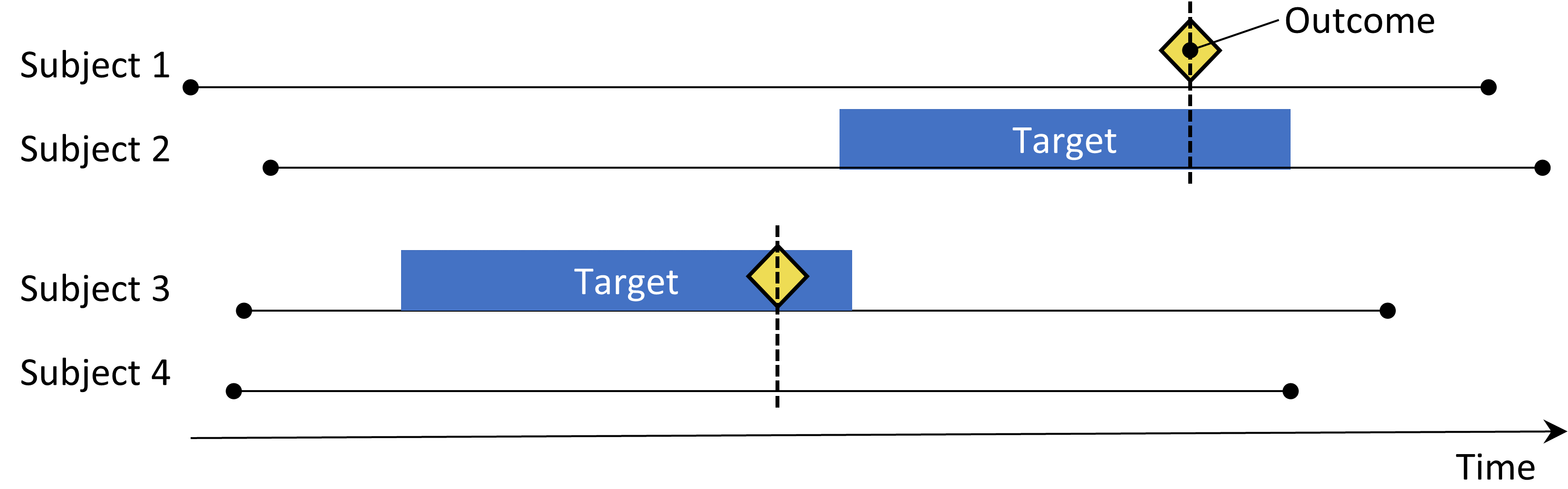
Figure 12.3: The case-control design. Subjects with the outcome (‘cases’) are compared to subjects without the outcome (‘controls’) in terms of their exposure status. Often, cases and controls are matched on various characteristics such as age and sex.
Case-control studies (Vandenbroucke and Pearce 2012) consider the question “are persons with a specific disease outcome exposed more frequently to a specific agent than those without the disease?” Thus, the central idea is to compare “cases,” i.e., subjects that experience the outcome of interest, with “controls,” i.e., subjects that did not experience the outcome of interest. The choices in Table 12.3 define a case-control question.
| Choice | Description |
|---|---|
| Outcome cohort | A cohort representing the cases (the outcome of interest) |
| Control cohort | A cohort representing the controls. Typically the control cohort is automatically derived from the outcome cohort using some selection logic |
| Target cohort | A cohort representing the treatment |
| Nesting cohort | Optionally, a cohort defining the subpopulation from which cases and controls are drawn |
| Time-at-risk | At what time (often relative to the index date) do we consider exposure status? |
Often, one selects controls to match cases based on characteristics such as age and sex to make them more comparable. Another widespread practice is to nest the analysis within a specific subgroup of people, for example people that have all been diagnosed with one of the indications of the exposure of interest.
12.4 The Case-Crossover Design
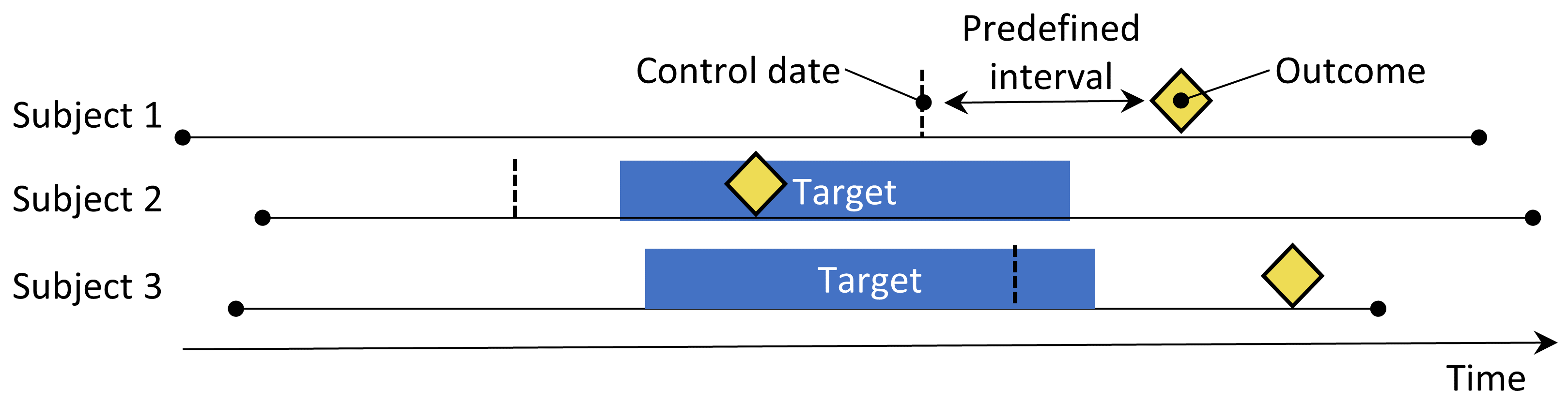
Figure 12.4: The case-crossover design. The time around the outcome is compared to a control date set at a predefined interval prior to the outcome date.
The case-crossover (Maclure 1991) design evaluates whether the rate of exposure is different at the time of the outcome than at some predefined number of days prior to the outcome. It is trying to determine whether there is something special about the day the outcome occurred. Table 12.4 shows the choices that define a case-crossover question.
| Choice | Description |
|---|---|
| Outcome cohort | A cohort representing the cases (the outcome of interest) |
| Target cohort | A cohort representing the treatment |
| Time-at-risk | At what time (often relative to the index date) do we consider exposure status? |
| Control time | The time period used as the control time |
Cases serve as their own controls. As self-controlled designs, they should be robust to confounding due to between-person differences. One concern is that, because the outcome date is always later than the control date, the method will be positively biased if the overall frequency of exposure increases over time (or negatively biased if there is a decrease). To address this, the case-time-control design (Suissa 1995) was developed, which adds controls, matched for example on age and sex, to the case-crossover design to adjust for exposure trends.
12.5 The Self-Controlled Case Series Design
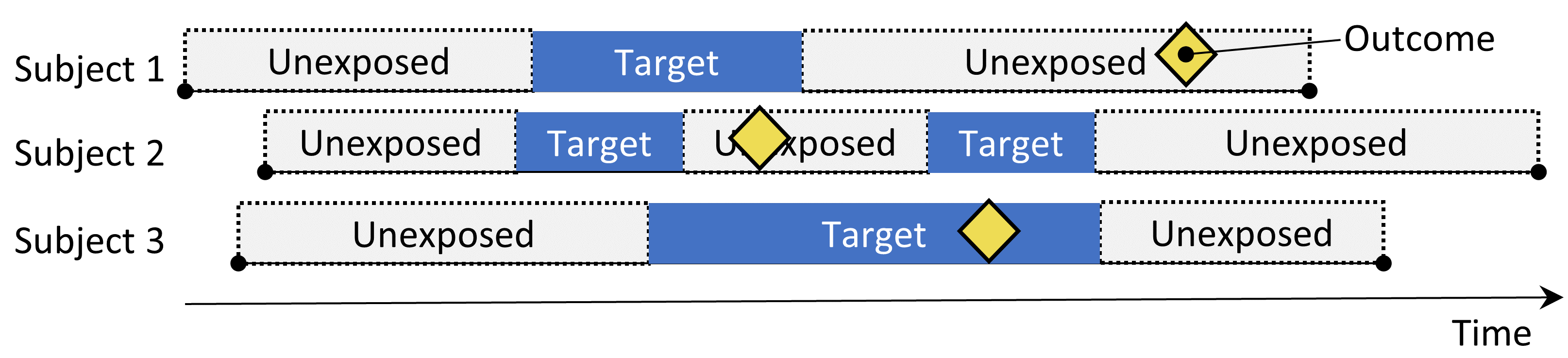
Figure 12.5: The Self-Controlled Case Series design. The rate of outcomes during exposure is compared to the rate of outcomes when not exposed.
The Self-Controlled Case Series (SCCS) design (Farrington 1995; Whitaker et al. 2006) compares the rate of outcomes during exposure to the rate of outcomes during all unexposed time, including before, between, and after exposures. It is a Poisson regression that is conditioned on the person. Thus, it seeks to answer the question: “Given that a patient has the outcome, is the outcome more likely during exposed time compared to non-exposed time?”. The choices in Table 12.5 define an SCCS question.
| Choice | Description |
|---|---|
| Target cohort | A cohort representing the treatment |
| Outcome cohort | A cohort representing the outcome of interest |
| Time-at-risk | At what time (often relative to the target cohort start and end dates) do we consider the risk of the outcome? |
| Model | The model to estimate the effect, including any adjustments for time-varying confounders |
Like other self-controlled designs, the SCCS is robust to confounding due to between-person differences, but vulnerable to confounding due to time-varying effects. Several adjustments are possible to attempt to account for these, for example by including age and season. A special variant of the SCCS includes not just the exposure of interest, but all other exposures to drugs recorded in the database (Simpson et al. 2013) potentially adding thousands of additional variables to the model. L1-regularization using cross-validation to select the regularization hyperparameter is applied to the coefficients of all exposures except the exposure of interest.
One important assumption underlying the SCCS is that the observation period end is independent of the date of the outcome. For some outcomes, especially ones that can be fatal such as stroke, this assumption can be violated. An extension to the SCCS has been developed that corrects for any such dependency. (Farrington et al. 2011)
12.6 Designing a Hypertension Study
12.6.1 Problem Definition
ACE inhibitors (ACEi) are widely used in patients with hypertension or ischemic heart disease, especially those with other comorbidities such as congestive heart failure, diabetes mellitus, or chronic kidney disease. (Zaman, Oparil, and Calhoun 2002) Angioedema, a serious and sometimes life-threatening adverse event that usually manifests as swelling of the lips, tongue, mouth, larynx, pharynx, or periorbital region, has been linked to the use of these medications. (Sabroe and Black 1997) However, limited information is available about the absolute and relative risks for angioedema associated with the use of these medications. Existing evidence is primarily based on investigations of specific cohorts (e.g., predominantly male veterans or Medicaid beneficiaries) whose findings may not be generalizable to other populations, or based on investigations with few events, which provide unstable risk estimates. (Powers et al. 2012) Several observational studies compare ACEi to beta-blockers for the risk of angioedema, (Magid et al. 2010; Toh et al. 2012) but beta-blockers are no longer recommended as first-line treatment of hypertension. (Whelton et al. 2018) A viable alternative treatment could be thiazides or thiazide-like diuretics (THZ), which could be just as effective in managing hypertension and its associated risks such as acute myocardial infarction (AMI), but without increasing the risk of angioedema.
The following will demonstrate how to apply our population-level estimation framework to observational healthcare data to address the following comparative estimation questions:
What is the risk of angioedema in new users of ACE inhibitors compared to new users of thiazide and thiazide-like diuretics?
What is the risk of acute myocardial infarction in new users of ACE inhibitors compared to new users of thiazide and thiazide-like diuretics?
Since these are comparative effect estimation questions we will apply the cohort method as described in Section 12.1.
12.6.2 Target and Comparator
We consider patients new-users if their first observed treatment for hypertension was monotherapy with any active ingredient in either the ACEi or THZ class. We define mono therapy as not starting on any other anti-hypertensive drug in the seven days following treatment initiation. We require patients to have at least one year of prior continuous observation in the database before first exposure and a recorded hypertension diagnosis at or in the year preceding treatment initiation.
12.6.3 Outcome
We define angioedema as any occurrence of an angioedema condition concept during an inpatient or emergency room (ER) visit, and require there to be no angioedema diagnosis recorded in the seven days prior. We define AMI as any occurrence of an AMI condition concept during an inpatient or ER visit, and require there to be no AMI diagnosis record in the 180 days prior.
12.6.4 Time-At-Risk
We define time-at-risk to start on the day after treatment initiation, and stop when exposure stops, allowing for a 30-day gap between subsequent drug exposures.
12.6.5 Model
We fit a PS model using the default set of covariates, including demographics, conditions, drugs, procedures, measurements, observations, and several co-morbidity scores. We exclude ACEi and THZ from the covariates. We perform variable-ratio matching and condition the Cox regression on the matched sets.
12.6.6 Study Summary
| Choice | Value |
|---|---|
| Target cohort | New users of ACE inhibitors as first-line monotherapy for hypertension. |
| Comparator cohort | New users of thiazides or thiazide-like diuretics as first-line monotherapy for hypertension. |
| Outcome cohort | Angioedema or acute myocardial infarction. |
| Time-at-risk | Starting the day after treatment initiation, stopping when exposure stops. |
| Model | Cox proportional hazards model using variable-ratio matching. |
12.6.7 Control Questions
To evaluate whether our study design produces estimates in line with the truth, we additionally include a set of control questions where the true effect size is known. Control questions can be divided in negative controls, having a hazard ratio of 1, and positive controls, having a known hazard ratio greater than 1. For several reasons we use real negative controls, and synthesize positive controls based on these negative controls. How to define and use control questions is discussed in detail in Chapter 18.
12.7 Implementing the Study Using ATLAS
Here we demonstrate how this study can be implemented using the Estimation function in ATLAS. Click on  in the left bar of ATLAS, and create a new estimation study. Make sure to give the study an easy-to-recognize name. The study design can be saved at any time by clicking the
  button.
In the Estimation design function, there are three sections: Comparisons, Analysis Settings, and Evaluation Settings. We can specify multiple comparisons and multiple analysis settings, and ATLAS will execute all combinations of these as separate analyses. Here we discuss each section:
12.7.1 Comparative Cohort Settings
A study can have one or more comparisons. Click on “Add Comparison,” which will open a new dialog. Click on  to select the target and comparator cohorts. By clicking on “Add Outcome” we can add our two outcome cohorts. We assume the cohorts have already been created in ATLAS as described in Chapter 10. The Appendix provides the full definitions of the target (Appendix B.2), comparator (Appendix B.5), and outcome (Appendix B.4 and Appendix B.3) cohorts. When done, the dialog should look like Figure 12.6.
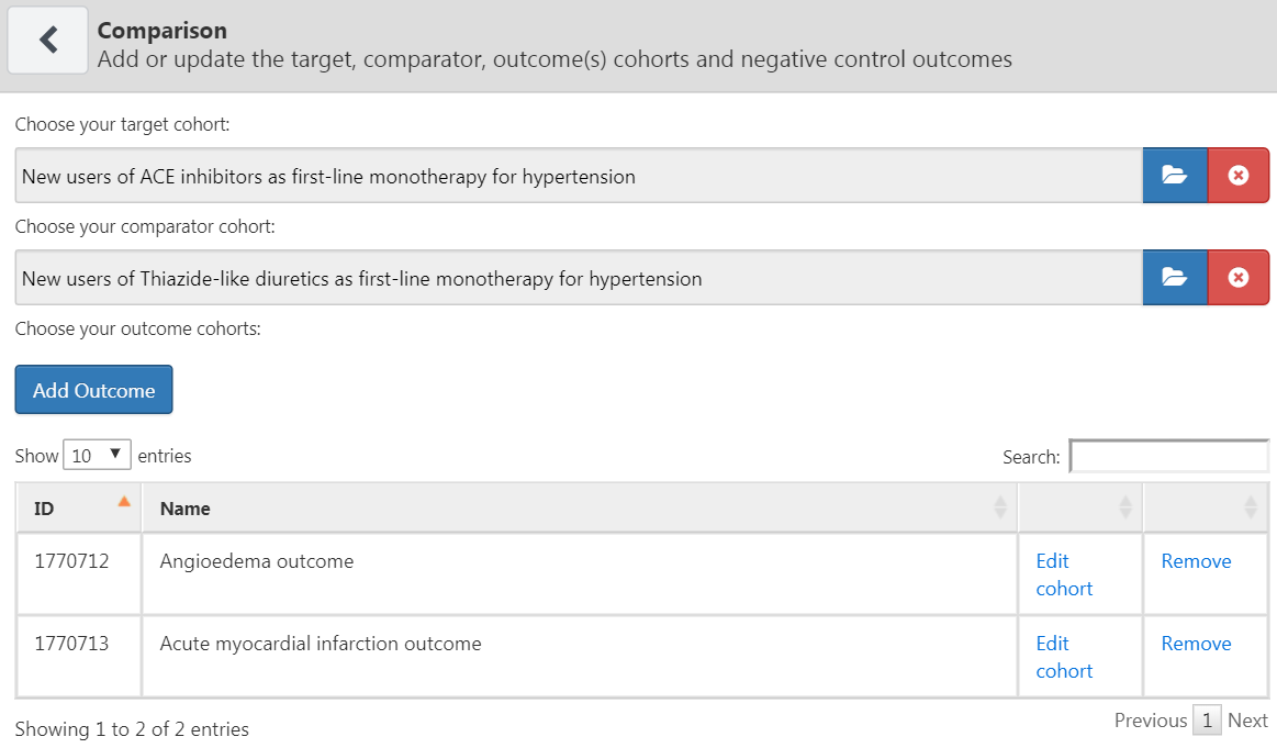
Figure 12.6: The comparison dialog
Note that we can select multiple outcomes for a target-comparator pair. Each outcome will be treated independently, and will result in a separate analysis.
Negative Control Outcomes
Negative control outcomes are outcomes that are not believed to be caused by either the target or the comparator, and where therefore the true hazard ratio equals 1. Ideally, we would have proper cohort definitions for each outcome cohort. However, typically, we only have a concept set, with one concept per negative control outcome, and some standard logic to turn these into outcome cohorts. Here we assume the concept set has already been created as described in Chapter 18 and can simply be selected. The negative control concept set should contain a concept per negative control, and not include descendants. Figure 12.7 shows the negative control concept set used for this study.
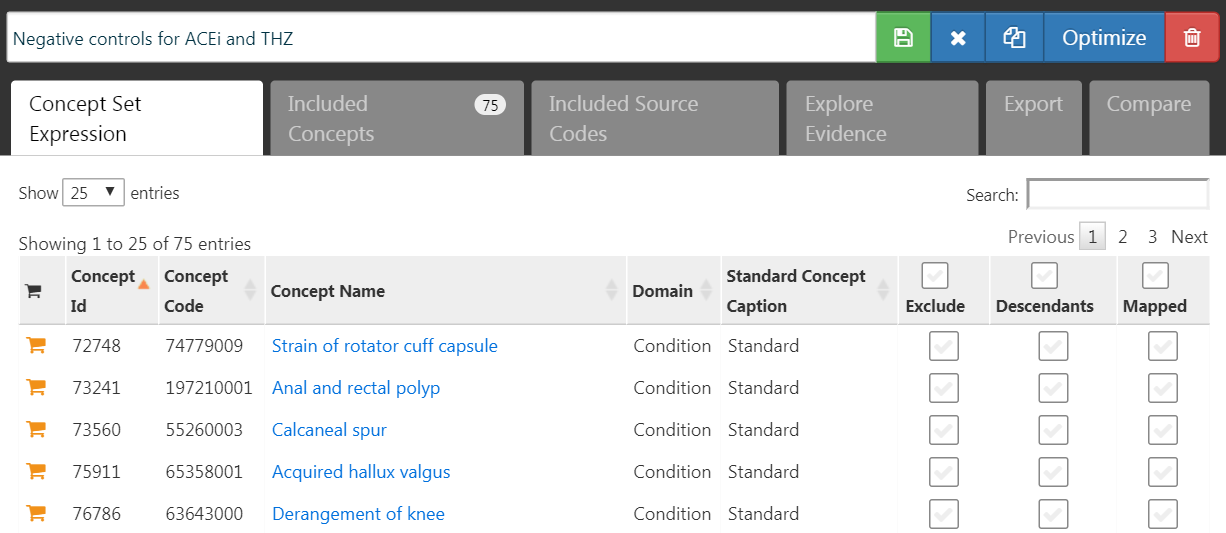
Figure 12.7: Negative Control concept set.
Concepts to Include
When selecting concept to include, we can specify which covariates we would like to generate, for example to use in a propensity model. When specifying covariates here, all other covariates (aside from those you specified) are left out. We usually want to include all baseline covariates, letting the regularized regression build a model that balances all covariates. The only reason we might want to specify particular covariates is to replicate an existing study that manually picked covariates. These inclusions can be specified in this comparison section or in the analysis section, because sometimes they pertain to a specific comparison (e.g. known confounders in a comparison), or sometimes they pertain to an analysis (e.g. when evaluating a particular covariate selection strategy).
Concepts to Exclude
Rather than specifying which concepts to include, we can instead specify concepts to exclude. When we submit a concept set in this field, we use every covariate except for those that we submitted. When using the default set of covariates, which includes all drugs and procedures occurring on the day of treatment initiation, we must exclude the target and comparator treatment, as well as any concepts that are directly related to these. For example, if the target exposure is an injectable, we should not only exclude the drug, but also the injection procedure from the propensity model. In this example, the covariates we want to exclude are ACEi and THZ. Figure 12.8 shows we select a concept set that includes all these concepts, including their descendants.
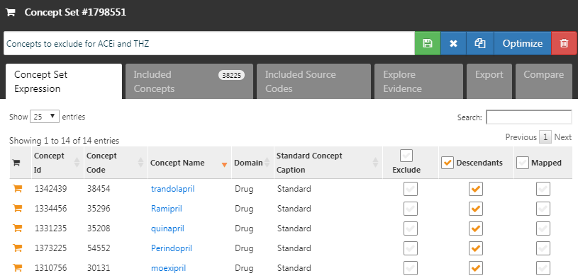
Figure 12.8: The concept set defining the concepts to exclude.
After selecting the negative controls and covariates to exclude, the lower half of the comparisons dialog should look like Figure 12.9.
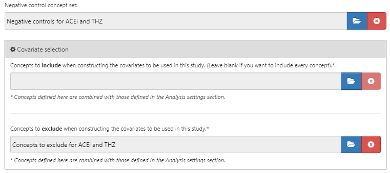
Figure 12.9: The comparison window showing concept sets for negative controls and concepts to exclude.
12.7.2 Effect Estimation Analysis Settings
After closing the comparisons dialog we can click on “Add Analysis Settings.” In the box labeled “Analysis Name,” we can give the analysis a unique name that is easy to remember and locate in the future. For example, we could set the name to “Propensity score matching.”
Study Population
There are a wide range of options to specify the study population, which is the set of subjects that will enter the analysis. Many of these overlap with options available when designing the target and comparator cohorts in the cohort definition tool. One reason for using the options in Estimation instead of in the cohort definition is re-usability; we can define the target, comparator, and outcome cohorts completely independently, and add dependencies between these at a later point in time. For example, if we wish to remove people who had the outcome before treatment initiation, we could do so in the definitions of the target and comparator cohort, but then we would need to create separate cohorts for every outcome! Instead, we can choose to have people with prior outcomes be removed in the analysis settings, and now we can reuse our target and comparator cohorts for our two outcomes of interest (as well as our negative control outcomes).
The study start and end dates can be used to limit the analyses to a specific period. The study end date also truncates risk windows, meaning no outcomes beyond the study end date will be considered. One reason for selecting a study start date might be that one of the drugs being studied is new and did not exist in an earlier time. Automatically adjusting for this can be done by answering “yes” to the question “Restrict the analysis to the period when both exposures are present in the data?”. Another reason to adjust study start and end dates might be that medical practice changed over time (e.g., due to a drug warning) and we are only interested in the time where medicine was practiced a specific way.
The option “Should only the first exposure per subject be included?” can be used to restrict to the first exposure per patient. Often this is already done in the cohort definition, as is the case in this example. Similarly, the option “The minimum required continuous observation time prior to index date for a person to be included in the cohort” is often already set in the cohort definition, and can therefore be left at 0 here. Having observed time (as defined in the OBSERVATION_PERIOD table) before the index date ensures that there is sufficient information about the patient to calculate a propensity score, and is also often used to ensure the patient is truly a new user, and therefore was not exposed before.
“Remove subjects that are in both the target and comparator cohort?” defines, together with the option “If a subject is in multiple cohorts, should time-at-risk be censored when the new time-at-risk starts to prevent overlap?” what happens when a subject is in both target and comparator cohorts. The first setting has three choices:
- “Keep All” indicating to keep the subjects in both cohorts. With this option it might be possible to double-count subjects and outcomes.
- “Keep First” indicating to keep the subject in the first cohort that occurred.
- “Remove All” indicating to remove the subject from both cohorts.
If the options “keep all” or “keep first” are selected, we may wish to censor the time when a person is in both cohorts. This is illustrated in Figure 12.10. By default, the time-at-risk is defined relative to the cohort start and end date. In this example, the time-at-risk starts one day after cohort entry, and stops at cohort end. Without censoring the time-at-risk for the two cohorts might overlap. This is especially problematic if we choose to keep all, because any outcome that occurs during this overlap (as shown) will be counted twice. If we choose to censor, the first cohort’s time-at-risk ends when the second cohort’s time-at-risk starts.
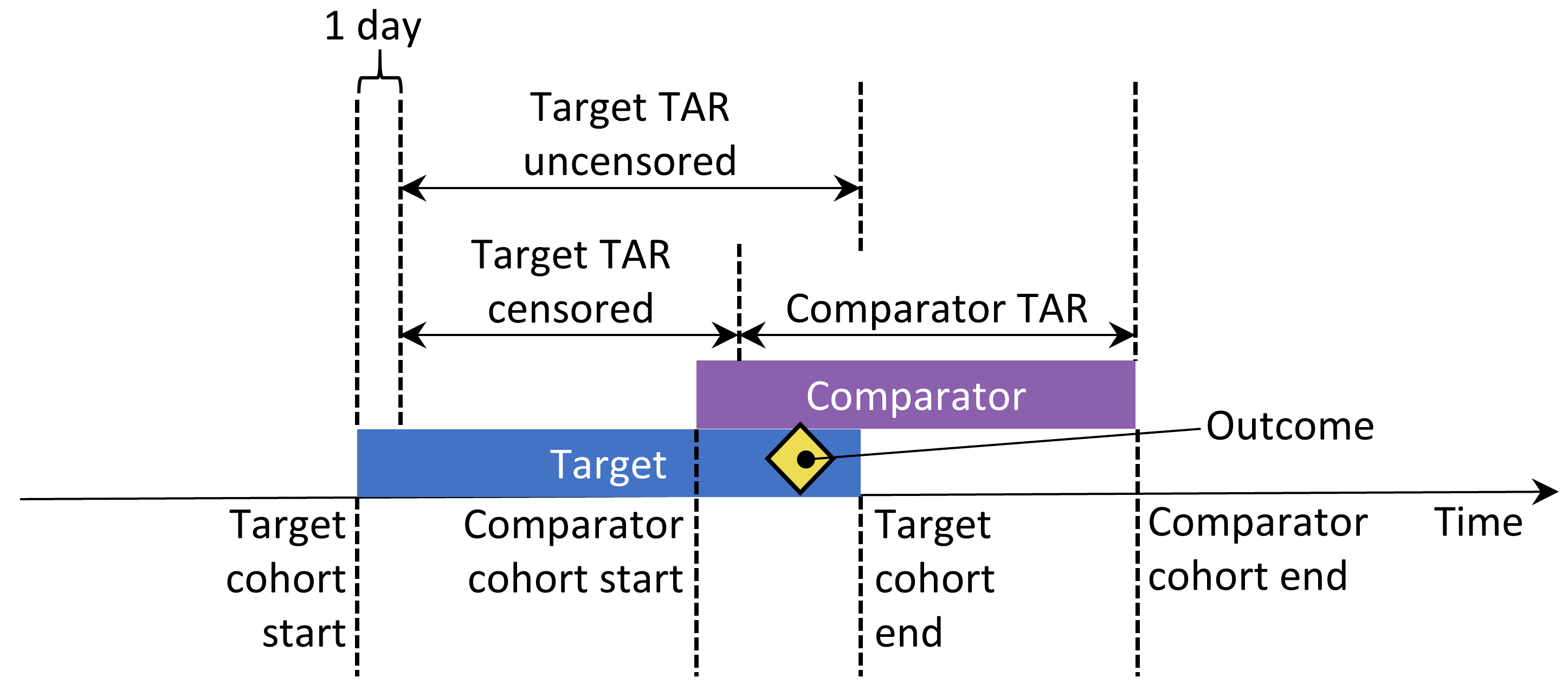
Figure 12.10: Time-at-risk (TAR) for subjects who are in both cohorts, assuming time-at-risk starts the day after treatment initiation, and stops at exposure end.
We can choose to remove subjects that have the outcome prior to the risk window start, because often a second outcome occurrence is the continuation of the first one. For instance, when someone develops heart failure, a second occurrence is likely, which means the heart failure probably never fully resolved in between. On the other hand, some outcomes are episodic, and it would be expected for patients to have more than one independent occurrence, like an upper respiratory infection. If we choose to remove people that had the outcome before, we can select how many days we should look back when identifying prior outcomes.
Our choices for our example study are shown in Figure 12.11. Because our target and comparator cohort definitions already restrict to the first exposure and require observation time prior to treatment initiation, we do not apply these criteria here.
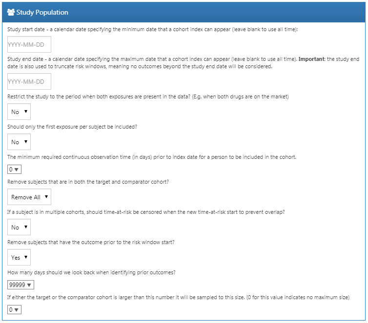
Figure 12.11: Study population settings.
Covariate Settings
Here we specify the covariates to construct. These covariates are typically used in the propensity model, but can also be included in the outcome model (the Cox proportional hazards model in this case). If we click to view details of our covariate settings, we can select which sets of covariates to construct. However, the recommendation is to use the default set, which constructs covariates for demographics, all conditions, drugs, procedures, measurements, etc.
We can modify the set of covariates by specifying concepts to include and/or exclude. These settings are the same as the ones found in Section 12.7.1 on comparison settings. The reason why they can be found in two places is because sometimes these settings are related to a specific comparison, as is the case here because we wish to exclude the drugs we are comparing, and sometimes the settings are related to a specific analysis. When executing an analysis for a specific comparison using specific analysis settings, the OHDSI tools will take the union of these sets.
Figure 12.12 shows our choices for this study. Note that we have selected to add descendants to the concept to exclude, which we defined in the comparison settings in Figure 12.9.
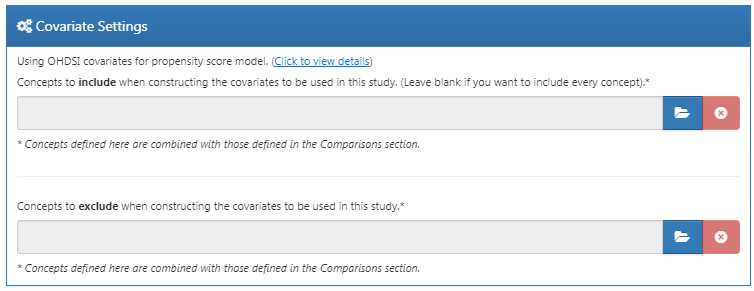
Figure 12.12: Covariate settings.
Time At Risk
Time-at-risk is defined relative to the start and end dates of our target and comparator cohorts. In our example, we had set the cohort start date to start on treatment initiation, and cohort end date when exposure stops (for at least 30 days). We set the start of time-at-risk to one day after cohort start, so one day after treatment initiation. A reason to set the time-at-risk start to be later than the cohort start is because we may want to exclude outcome events that occur on the day of treatment initiation if we do not believe it biologically plausible they can be caused by the drug.
We set the end of the time-at-risk to the cohort end, so when exposure stops. We could choose to set the end date later if for example we believe events closely following treatment end may still be attributable to the exposure. In the extreme we could set the time-at-risk end to a large number of days (e.g. 99999) after the cohort end date, meaning we will effectively follow up subjects until observation end. Such a design is sometimes referred to as an intent-to-treat design.
A patient with zero days at risk adds no information, so the minimum days at risk is normally set at one day. If there is a known latency for the side effect, then this may be increased to get a more informative proportion. It can also be used to create a cohort more similar to that of a randomized trial it is being compared to (e.g., all the patients in the randomized trial were observed for at least N days).
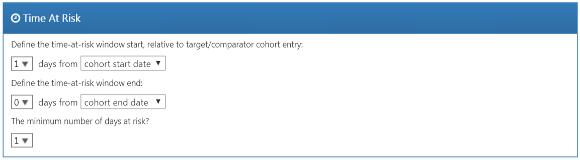
Figure 12.13: Time-at-risk settings.
Propensity Score Adjustment
We can opt to trim the study population, removing people with extreme PS values. We can choose to remove the top and bottom percentage, or we can remove subjects whose preference score falls outside the range we specify. Trimming the cohorts is generally not recommended because it requires discarding observations, which reduces statistical power. It may be desirable to trim in some cases, for example when using IPTW.
In addition to, or instead of trimming, we can choose to stratify or match on the propensity score. When stratifying we need to specify the number of strata and whether to select the strata based on the target, comparator, or entire study population. When matching we need to specify the maximum number of people from the comparator group to match to each person in the target group. Typical values are 1 for one-on-one matching, or a large number (e.g. 100) for variable-ratio matching. We also need to specify the caliper: the maximum allowed difference between propensity scores to allow a match. The caliper can be defined on difference caliper scales:
- The propensity score scale: the PS itself
- The standardized scale: in standard deviations of the PS distributions
- The standardized logit scale: in standard deviations of the PS distributions after the logit transformation to make the PS more normally distributed.
In case of doubt, we suggest using the default values, or consult the work on this topic by Austin (2011).
Fitting large-scale propensity models can be computationally expensive, so we may want to restrict the data used to fit the model to just a sample of the data. By default the maximum size of the target and comparator cohort is set to 250,000. In most studies this limit will not be reached. It is also unlikely that more data will lead to a better model. Note that although a sample of the data may be used to fit the model, the model will be used to compute PS for the entire population.
Test each covariate for correlation with the target assignment? If any covariate has an unusually high correlation (either positive or negative), this will throw an error. This avoids lengthy calculation of a propensity model only to discover complete separation. Finding very high univariate correlation allows you to review the covariate to determine why it has high correlation and whether it should be dropped.
Use regularization when fitting the model? The standard procedure is to include many covariates (typically more than 10,000) in the propensity model. In order to fit such models some regularization is required. If only a few hand-picked covariates are included, it is also possible to fit the model without regularization.
Figure 12.14 shows our choices for this study. Note that we select variable-ratio matching by setting the maximum number of people to match to 100.
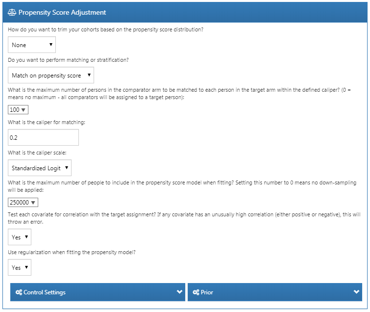
Figure 12.14: Propensity score adjustment settings.
Outcome Model Settings
First, we need to specify the statistical model we will use to estimate the relative risk of the outcome between target and comparator cohorts. We can choose between Cox, Poisson, and logistic regression, as discussed briefly in Section 12.1. For our example we choose a Cox proportional hazards model, which considers time to first event with possible censoring. Next, we need to specify whether the regression should be conditioned on the strata. One way to understand conditioning is to imagine a separate estimate is produced in each stratum, and then combined across strata. For one-to-one matching this is likely unnecessary and would just lose power. For stratification or variable-ratio matching it is required.
We can also choose to add the covariates to the outcome model to adjust the analysis. This can be done in addition or instead of using a propensity model. However, whereas there usually is ample data to fit a propensity model, with many people in both treatment groups, there is typically very little data to fit the outcome model, with only few people having the outcome. We therefore recommend keeping the outcome model as simple as possible and not include additional covariates.
Instead of stratifying or matching on the propensity score we can also choose to use inverse probability of treatment weighting (IPTW).
If we choose to include all covariates in the outcome model, it may make sense to use regularization when fitting the model if there are many covariates. Note that no regularization will be applied to the treatment variable to allow for unbiased estimation.
Figure 12.15 shows our choices for this study. Because we use variable-ratio matching, we must condition the regression on the strata (i.e. the matched sets).
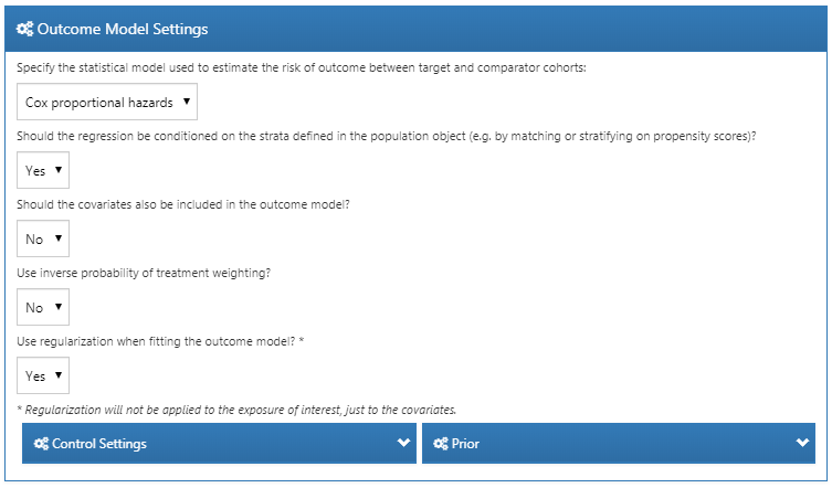
Figure 12.15: Outcome model settings.
12.7.3 Evaluation Settings
As described in Chapter 18, negative and positive controls should be included in our study to evaluate the operating characteristics, and perform empirical calibration.
Negative Control Outcome Cohort Definition
In Section 12.7.1 we selected a concept set representing the negative control outcomes. However, we need logic to convert concepts to cohorts to be used as outcomes in our analysis. ATLAS provides standard logic with three choices. The first choice is whether to use all occurrences or just the first occurrence of the concept. The second choice determines whether occurrences of descendant concepts should be considered. For example, occurrences of the descendant “ingrown nail of foot” can also be counted as an occurrence of the ancestor “ingrown nail.” The third choice specifies which domains should be considered when looking for the concepts.
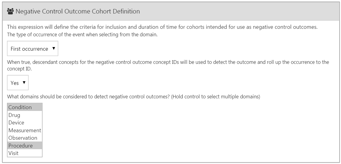
Figure 12.16: Negative control outcome cohort definition settings.
Positive Control Synthesis
In addition to negative controls we can also include positive controls, which are exposure-outcome pairs where a causal effect is believed to exist with known effect size. For various reasons real positive controls are problematic, so instead we rely on synthetic positive controls, derived from negative controls as described in Chapter 18. We can choose to perform positive control synthesis. If “yes”, we must choose the model type, currently being “Poisson” and “survival”. Since we use a survival (Cox) model in our estimation study, we should choose “survival”. We define the time-at-risk model for the positive control synthesis to be the same as in our estimation settings, and similarly mimic the choices for the minimum required continuous observation prior to exposure, should only the first exposure be included, should only the first outcome be included, as well as remove people with prior outcomes. Figure 12.15 shows the settings for the positive control synthesis.
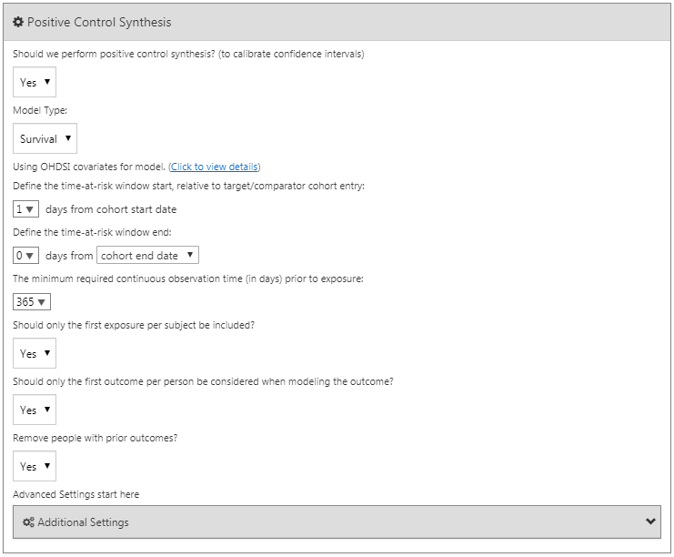
Figure 12.17: Negative control outcome cohort definition settings.
12.7.4 Running the Study Package
Now that we have fully defined our study, we can export it as an executable R package. This package contains everything that is needed to execute the study at a site that has data in CDM. This includes the cohort definitions that can be used to instantiate the target, comparator and outcome cohorts, the negative control concept set and logic to create the negative control outcome cohorts, as well as the R code to execute the analysis. Before generating the package make sure to save your study, then click on the Utilities tab. Here we can review the set of analyses that will be performed. As mentioned before, every combination of a comparison and an analysis setting will result in a separate analysis. In our example we have specified two analyses: ACEi versus THZ for AMI, and ACEi versus THZ for angioedema, both using propensity score matching.
We must provide a name for our package, after which we can click on “Download” to download the zip file. The zip file contains an R package, with the usual required folder structure for R packages. (Wickham 2015) To use this package we recommend using R Studio. If you are running R Studio locally, unzip the file, and double click the .Rproj file to open it in R Studio. If you are running R Studio on an R studio server, click  to upload and unzip the file, then click on the .Rproj file to open the project.
Once you have opened the project in R Studio, you can open the README file, and follow the instructions. Make sure to change all file paths to existing paths on your system.
A common error message that may appear when running the study is “High correlation between covariate(s) and treatment detected.” This indicates that when fitting the propensity model, some covariates were observed to be highly correlated with the exposure. Please review the covariates mentioned in the error message, and exclude them from the set of covariates if appropriate (see Section 12.1.2).
12.8 Implementing the Study Using R
Instead of using ATLAS to write the R code that executes the study, we can also write the R code ourselves. One reason we might want to do this is because R offers far greater flexibility than is exposed in ATLAS. If we for example wish to use custom covariates, or a linear outcome model, we will need to write some custom R code, and combine it with the functionality provided by the OHDSI R packages.
For our example study we will rely on the CohortMethod package to execute our study. CohortMethod extracts the necessary data from a database in the CDM and can use a large set of covariates for the propensity model. In the following example we first only consider angioedema as outcome. In Section 12.8.6 we then describe how this can be extended to include AMI and the negative control outcomes.
12.8.1 Cohort Instantiation
We first need to instantiate the target and outcome cohorts. Instantiating cohorts is described in Chapter 10. The Appendix provides the full definitions of the target (Appendix B.2), comparator (Appendix B.5), and outcome (Appendix B.4 ) cohorts. We will assume the ACEi, THZ, and angioedema cohorts have been instantiated in a table called scratch.my_cohorts with cohort definition IDs 1, 2, and 3 respectively.
12.8.2 Data Extraction
We first need to tell R how to connect to the server. CohortMethod uses the DatabaseConnector package, which provides a function called createConnectionDetails. Type ?createConnectionDetails for the specific settings required for the various database management systems (DBMS). For example, one might connect to a PostgreSQL database using this code:
library(CohortMethod)
connDetails <- createConnectionDetails(dbms = "postgresql",
                                       server = "localhost/ohdsi",
                                       user = "joe",
                                       password = "supersecret")

cdmDbSchema <- "my_cdm_data"
cohortDbSchema <- "scratch"
cohortTable <- "my_cohorts"
cdmVersion <- "5"
The last four lines define the cdmDbSchema, cohortDbSchema, and cohortTable variables, as well as the CDM version. We will use these later to tell R where the data in CDM format live, where the cohorts of interest have been created, and what version CDM is used. Note that for Microsoft SQL Server, database schemas need to specify both the database and the schema, so for example cdmDbSchema <- "my_cdm_data.dbo".
Now we can tell CohortMethod to extract the cohorts, construct covariates, and extract all necessary data for our analysis:
# target and comparator ingredient concepts:
aceI <- c(1335471,1340128,1341927,1363749,1308216,1310756,1373225,
          1331235,1334456,1342439)
thz <- c(1395058,974166,978555,907013)

# Define which types of covariates must be constructed:
cs <- createDefaultCovariateSettings(excludedCovariateConceptIds = c(aceI,
                                                                     thz),
                                     addDescendantsToExclude = TRUE)

#Load data:
cmData <- getDbCohortMethodData(connectionDetails = connectionDetails,
                                cdmDatabaseSchema = cdmDatabaseSchema,
                                oracleTempSchema = NULL,
                                targetId = 1,
                                comparatorId = 2,
                                outcomeIds = 3,
                                studyStartDate = "",
                                studyEndDate = "",
                                exposureDatabaseSchema = cohortDbSchema,
                                exposureTable = cohortTable,
                                outcomeDatabaseSchema = cohortDbSchema,
                                outcomeTable = cohortTable,
                                cdmVersion = cdmVersion,
                                firstExposureOnly = FALSE,
                                removeDuplicateSubjects = FALSE,
                                restrictToCommonPeriod = FALSE,
                                washoutPeriod = 0,
                                covariateSettings = cs)
cmData
## CohortMethodData object
##
## Treatment concept ID: 1
## Comparator concept ID: 2
## Outcome concept ID(s): 3There are many parameters, but they are all documented in the CohortMethod manual. The createDefaultCovariateSettings function is described in the FeatureExtraction package. In short, we are pointing the function to the table containing our cohorts and specify which cohort definition IDs in that table identify the target, comparator and outcome. We instruct that the default set of covariates should be constructed, including covariates for all conditions, drug exposures, and procedures that were found on or before the index date. As mentioned in Section 12.1 we must exclude the target and comparator treatments from the set of covariates, and here we achieve this by listing all ingredients in the two classes, and tell FeatureExtraction to also exclude all descendants, thus excluding all drugs that contain these ingredients.
All data about the cohorts, outcomes, and covariates are extracted from the server and stored in the cohortMethodData object. This object uses the package ff to store information in a way that ensures R does not run out of memory, even when the data are large, as mentioned in Section 8.4.2.
We can use the generic summary() function to view some more information of the data we extracted:
## CohortMethodData object summary
##
## Treatment concept ID: 1
## Comparator concept ID: 2
## Outcome concept ID(s): 3
##
## Treated persons: 67166
## Comparator persons: 35333
##
## Outcome counts:
##          Event count Person count
## 3               980          891
##
## Covariates:
## Number of covariates: 58349
## Number of non-zero covariate values: 24484665
Creating the cohortMethodData file can take considerable computing time, and it is probably a good idea to save it for future sessions. Because cohortMethodData uses ff, we cannot use R’s regular save function. Instead, we’ll have to use the saveCohortMethodData() function:
We can use the loadCohortMethodData() function to load the data in a future session.
Defining New Users
Typically, a new user is defined as first time use of a drug (either target or comparator), and typically a washout period (a minimum number of days prior to first use) is used to increase the probability that it is truly first use. When using the CohortMethod package, you can enforce the necessary requirements for new use in three ways:
- When defining the cohorts.
- When loading the cohorts using the
getDbCohortMethodDatafunction, you can use thefirstExposureOnly,removeDuplicateSubjects,restrictToCommonPeriod, andwashoutPeriodarguments. - When defining the study population using the
createStudyPopulationfunction (see below).
The advantage of option 1 is that the input cohorts are already fully defined outside of the CohortMethod package, and external cohort characterization tools can be used on the same cohorts used in this analysis. The advantage of options 2 and 3 is that they save you the trouble of limiting to first use yourself, for example allowing you to directly use the DRUG_ERA table in the CDM. Option 2 is more efficient than 3, since only data for first use will be fetched, while option 3 is less efficient but allows you to compare the original cohorts to the study population.
12.8.3 Defining the Study Population
Typically, the exposure cohorts and outcome cohorts will be defined independently of each other. When we want to produce an effect size estimate, we need to further restrict these cohorts and put them together, for example by removing exposed subjects that had the outcome prior to exposure, and only keeping outcomes that fall within a defined risk window. For this we can use the createStudyPopulation function:
studyPop <- createStudyPopulation(cohortMethodData = cmData,
                                  outcomeId = 3,
                                  firstExposureOnly = FALSE,
                                  restrictToCommonPeriod = FALSE,
                                  washoutPeriod = 0,
                                  removeDuplicateSubjects = "remove all",
                                  removeSubjectsWithPriorOutcome = TRUE,
                                  minDaysAtRisk = 1,
                                  riskWindowStart = 1,
                                  startAnchor = "cohort start",
                                  riskWindowEnd = 0,
                                  endAnchor = "cohort end")
Note that we’ve set firstExposureOnly and removeDuplicateSubjects to FALSE, and washoutPeriod to 0 because we already applied those criteria in the cohort definitions. We specify the outcome ID we will use, and that people with outcomes prior to the risk window start date will be removed. The risk window is defined as starting on the day after the cohort start date (riskWindowStart = 1 and startAnchor = "cohort start"), and the risk windows ends when the cohort exposure ends (riskWindowEnd = 0 and endAnchor = "cohort end"), which was defined as the end of exposure in the cohort definition. Note that the risk windows are automatically truncated at the end of observation or the study end date. We also remove subjects who have no time at risk. To see how many people are left in the study population we can always use the getAttritionTable function:
##                    description targetPersons comparatorPersons ...
## 1             Original cohorts         67212             35379 ...
## 2 Removed subs in both cohorts         67166             35333 ...
## 3             No prior outcome         67061             35238 ...
## 4 Have at least 1 days at risk         66780             35086 ...
12.8.4 Propensity Scores
We can fit a propensity model using the covariates constructed by getDbcohortMethodData(), and compute a PS for each person:
The createPs function uses the Cyclops package to fit a large-scale regularized logistic regression. To fit the propensity model, Cyclops needs to know the hyperparameter value which specifies the variance of the prior. By default Cyclops will use cross-validation to estimate the optimal hyperparameter. However, be aware that this can take a really long time. You can use the prior and control parameters of the createPs function to specify Cyclops’ behavior, including using multiple CPUs to speed-up the cross-validation.
Here we use the PS to perform variable-ratio matching:
matchedPop <- matchOnPs(population = ps, caliper = 0.2,
                        caliperScale = "standardized logit", maxRatio = 100)
Alternatively, we could have used the PS in the trimByPs, trimByPsToEquipoise, or stratifyByPs functions.
12.8.5 Outcome Models
The outcome model is a model describing which variables are associated with the outcome. Under strict assumptions, the coefficient for the treatment variable can be interpreted as the causal effect. In this case we fit a Cox proportional hazards model, conditioned (stratified) on the matched sets:
outcomeModel <- fitOutcomeModel(population = matchedPop,
                                modelType = "cox",
                                stratified = TRUE)
outcomeModel
## Model type: cox
## Stratified: TRUE
## Use covariates: FALSE
## Use inverse probability of treatment weighting: FALSE
## Status: OK
##
## Estimate lower .95 upper .95 logRr seLogRr
## treatment 4.3203 2.4531 8.0771 1.4633 0.30412.8.6 Running Multiple Analyses
Often we want to perform more than one analysis, for example for multiple outcomes including negative controls. The CohortMethod offers functions for performing such studies efficiently. This is described in detail in the package vignette on running multiple analyses. Briefly, assuming the outcome of interest and negative control cohorts have already been created, we can specify all target-comparator-outcome combinations we wish to analyze:
# Outcomes of interest:
ois <- c(3, 4) # Angioedema, AMI

# Negative controls:
ncs <- c(434165,436409,199192,4088290,4092879,44783954,75911,137951,77965,
         376707,4103640,73241,133655,73560,434327,4213540,140842,81378,
         432303,4201390,46269889,134438,78619,201606,76786,4115402,
         45757370,433111,433527,4170770,4092896,259995,40481632,4166231,
         433577,4231770,440329,4012570,4012934,441788,4201717,374375,
         4344500,139099,444132,196168,432593,434203,438329,195873,4083487,
         4103703,4209423,377572,40480893,136368,140648,438130,4091513,
         4202045,373478,46286594,439790,81634,380706,141932,36713918,
         443172,81151,72748,378427,437264,194083,140641,440193,4115367)

tcos <- createTargetComparatorOutcomes(targetId = 1,
                                       comparatorId = 2,
                                       outcomeIds = c(ois, ncs))

tcosList <- list(tcos)
Next, we specify what arguments should be used when calling the various functions described previously in our example with one outcome:
aceI <- c(1335471,1340128,1341927,1363749,1308216,1310756,1373225,
          1331235,1334456,1342439)
thz <- c(1395058,974166,978555,907013)

cs <- createDefaultCovariateSettings(excludedCovariateConceptIds = c(aceI,
                                                                     thz),
                                     addDescendantsToExclude = TRUE)

cmdArgs <- createGetDbCohortMethodDataArgs(
  studyStartDate = "",
  studyEndDate = "",
  firstExposureOnly = FALSE,
  removeDuplicateSubjects = FALSE,
  restrictToCommonPeriod = FALSE,
  washoutPeriod = 0,
  covariateSettings = cs)

spArgs <- createCreateStudyPopulationArgs(
  firstExposureOnly = FALSE,
  restrictToCommonPeriod = FALSE,
  washoutPeriod = 0,
  removeDuplicateSubjects = "remove all",
  removeSubjectsWithPriorOutcome = TRUE,
  minDaysAtRisk = 1,
  startAnchor = "cohort start",
  addExposureDaysToStart = FALSE,
  endAnchor = "cohort end",
  addExposureDaysToEnd = TRUE)

psArgs <- createCreatePsArgs()

matchArgs <- createMatchOnPsArgs(
  caliper = 0.2,
  caliperScale = "standardized logit",
  maxRatio = 100)

fomArgs <- createFitOutcomeModelArgs(
  modelType = "cox",
  stratified = TRUE)
We then combine these into a single analysis settings object, which we provide a unique analysis ID and some description. We can combine one or more analysis settings objects into a list:
cmAnalysis <- createCmAnalysis(
  analysisId = 1,
  description = "Propensity score matching",
  getDbCohortMethodDataArgs = cmdArgs,
  createStudyPopArgs = spArgs,
  createPs = TRUE,
  createPsArgs = psArgs,
  matchOnPs = TRUE,
  matchOnPsArgs = matchArgs
  fitOutcomeModel = TRUE,
  fitOutcomeModelArgs = fomArgs)

cmAnalysisList <- list(cmAnalysis)
We can now run the study including all comparisons and analysis settings:
result <- runCmAnalyses(connectionDetails = connectionDetails,
                        cdmDatabaseSchema = cdmDatabaseSchema,
                        exposureDatabaseSchema = cohortDbSchema,
                        exposureTable = cohortTable,
                        outcomeDatabaseSchema = cohortDbSchema,
                        outcomeTable = cohortTable,
                        cdmVersion = cdmVersion,
                        outputFolder = outputFolder,
                        cmAnalysisList = cmAnalysisList,
                        targetComparatorOutcomesList = tcosList)
The result object contains references to all the artifacts that were created. For example, we can retrieve the outcome model for AMI:
omFile <- result$outcomeModelFile[result$targetId == 1 &
                                    result$comparatorId == 2 &
                                    result$outcomeId == 4 &
                                    result$analysisId == 1]
outcomeModel <- readRDS(file.path(outputFolder, omFile))
outcomeModel
## Model type: cox
## Stratified: TRUE
## Use covariates: FALSE
## Use inverse probability of treatment weighting: FALSE
## Status: OK
##
## Estimate lower .95 upper .95 logRr seLogRr
## treatment 1.1338 0.5921 2.1765 0.1256 0.332We can also retrieve the effect size estimates for all outcomes with one command:
##     analysisId targetId comparatorId outcomeId        rr ...
## 1            1        1            2     72748 0.9734698 ...
## 2            1        1            2     73241 0.7067981 ...
## 3            1        1            2     73560 1.0623951 ...
## 4            1        1            2     75911 0.9952184 ...
## 5            1        1            2     76786 1.0861746 ...
## 6            1        1            2     77965 1.1439772 ...
12.9 Study Outputs
Our estimates are only valid if several assumptions have been met. We use a wide set of diagnostics to evaluate whether this is the case. These are available in the results produced by the R package generated by ATLAS, or can be generated on the fly using specific R functions.
12.9.1 Propensity Scores and Model
We first need to evaluate whether the target and comparator cohort are to some extent comparable. For this we can compute the Area Under the Receiver Operator Curve (AUC) statistic for the propensity model. An AUC of 1 indicates the treatment assignment was completely predictable based on baseline covariates, and that the two groups are therefore incomparable. We can use the computePsAuc function to compute the AUC, which in our example is 0.79. Using the plotPs function, we can also generate the preference score distribution as shown in Figure 12.18. Here we see that for many people the treatment they received was predictable, but there is also a large amount of overlap, indicating that adjustment can be used to select comparable groups.
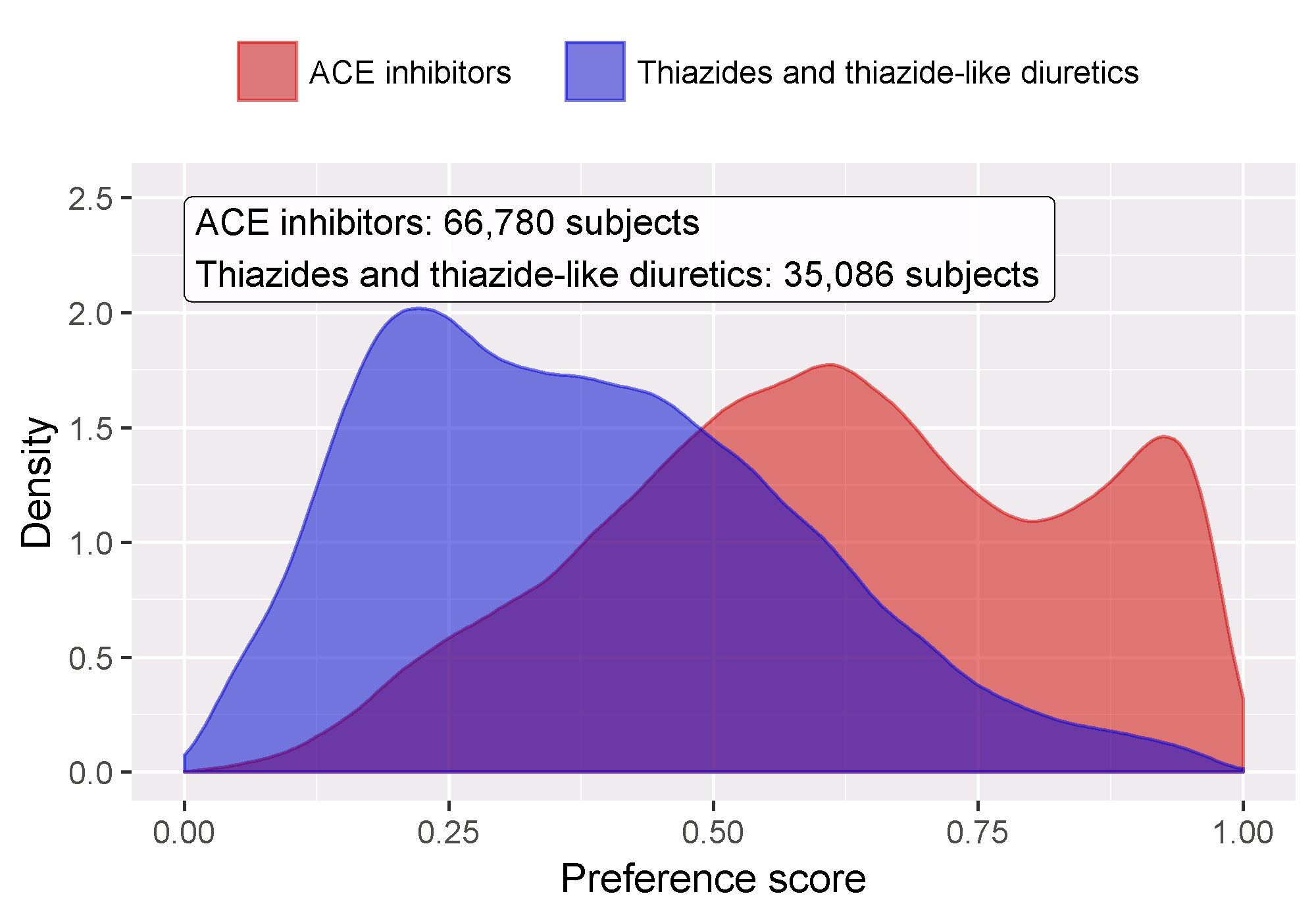
Figure 12.18: Preference score distribution.
In general it is a good idea to also inspect the propensity model itself, and especially so if the model is very predictive. That way we may discover which variables are most predictive. Table 12.7 shows the top predictors in our propensity model. Note that if a variable is too predictive, the CohortMethod package will throw an informative error rather than attempt to fit a model that is already known to be perfectly predictive.
| Beta | Covariate |
|---|---|
| -1.42 | condition_era group during day -30 through 0 days relative to index: Edema |
| -1.11 | drug_era group during day 0 through 0 days relative to index: Potassium Chloride |
| 0.68 | age group: 05-09 |
| 0.64 | measurement during day -365 through 0 days relative to index: Renin |
| 0.63 | condition_era group during day -30 through 0 days relative to index: Urticaria |
| 0.57 | condition_era group during day -30 through 0 days relative to index: Proteinuria |
| 0.55 | drug_era group during day -365 through 0 days relative to index: INSULINS AND ANALOGUES |
| -0.54 | race = Black or African American |
| 0.52 | (Intercept) |
| 0.50 | gender = MALE |
12.9.2 Covariate Balance
The goal of using PS is to make the two groups comparable (or at least to select comparable groups). We must verify whether this is achieved, for example by checking whether the baseline covariates are indeed balanced after adjustment. We can use the computeCovariateBalance and plotCovariateBalanceScatterPlot functions to generate Figure 12.19. One rule-of-thumb to use is that no covariate may have an absolute standardized difference of means greater than 0.1 after propensity score adjustment. Here we see that although there was substantial imbalance before matching, after matching we meet this criterion.
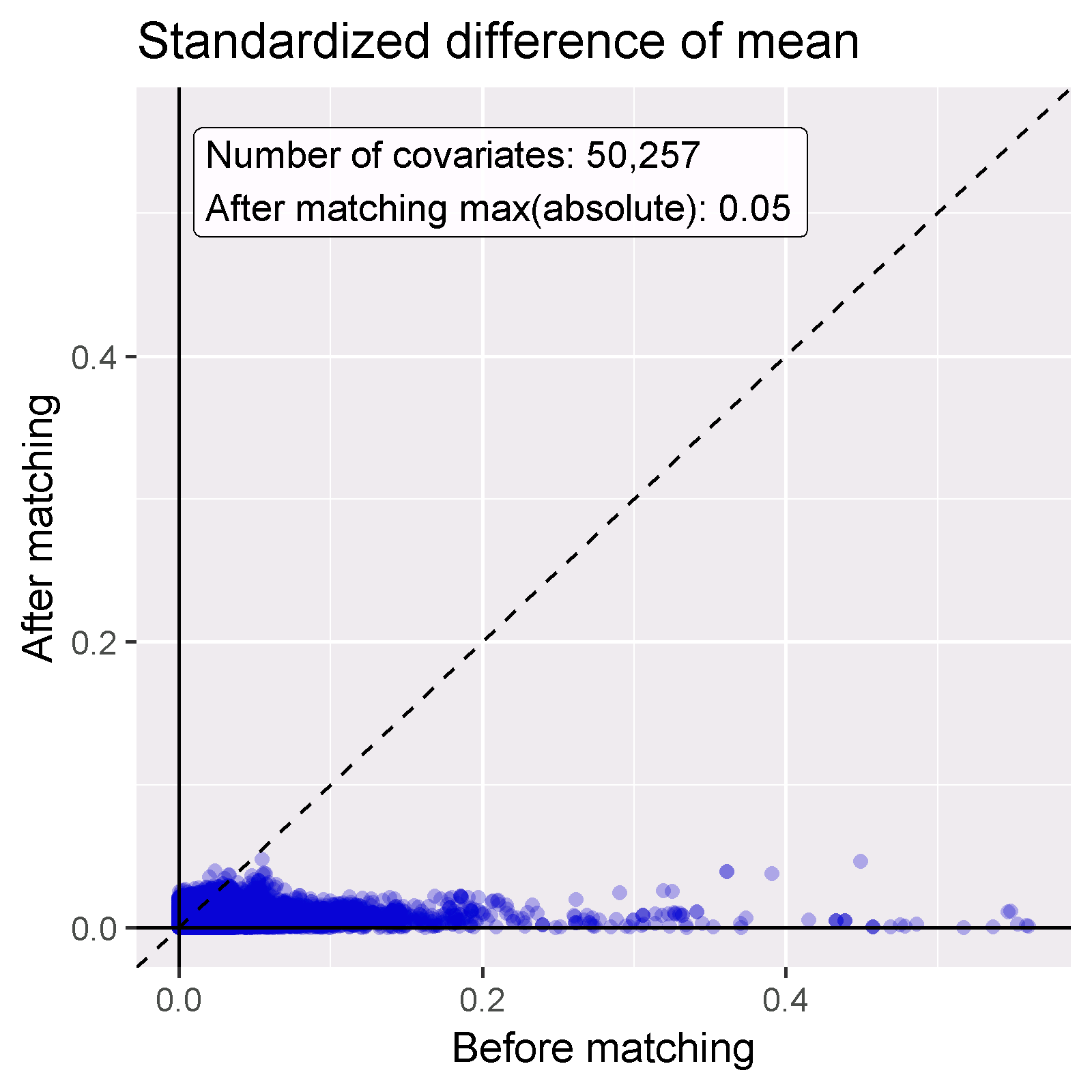
Figure 12.19: Covariate balance, showing the absolute standardized difference of mean before and after propensity score matching. Each dot represents a covariate.
12.9.3 Follow Up and Power
Before fitting an outcome model, we might be interested to know whether we have sufficient power to detect a particular effect size. It makes sense to perform these power calculations once the study population has been fully defined, so taking into account loss to the various inclusion and exclusion criteria (such as no prior outcomes), and loss due to matching and/or trimming. We can view the attrition of subjects in our study using the drawAttritionDiagram function as shown in Figure 12.20.
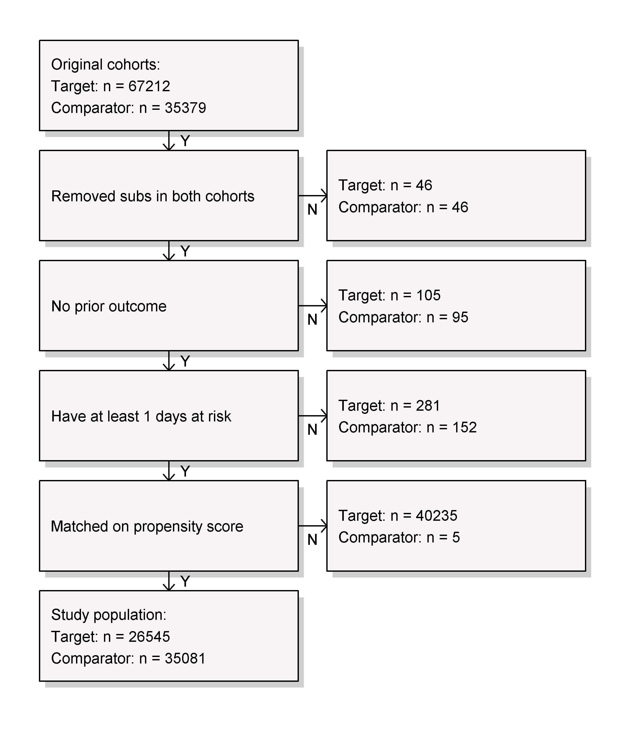
Figure 12.20: Attrition diagram. The counts shown at the top are those that meet our target and comparator cohort definitions. The counts at the bottom are those that enter our outcome model, in this case a Cox regression.
Since the sample size is fixed in retrospective studies (the data has already been collected), and the true effect size is unknown, it is therefore less meaningful to compute the power given an expected effect size. Instead, the CohortMethod package provides the computeMdrr function to compute the minimum detectable relative risk (MDRR). In our example study the MDRR is 1.69.
To gain a better understanding of the amount of follow-up available we can also inspect the distribution of follow-up time. We defined follow-up time as time at risk, so not censored by the occurrence of the outcome. The getFollowUpDistribution can provide a simple overview as shown in Figure 12.21, which suggests the follow-up time for both cohorts is comparable.
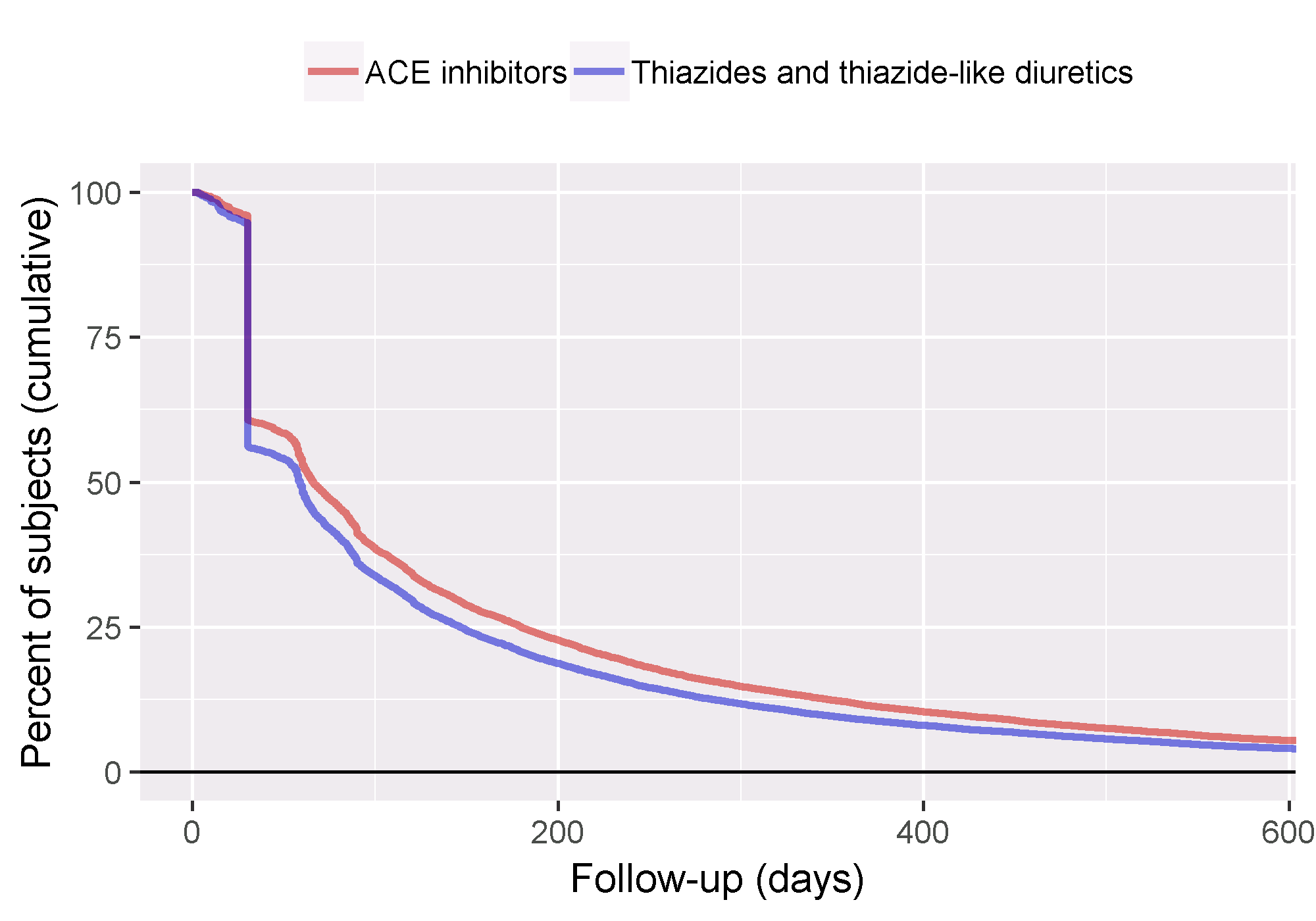
Figure 12.21: Distribution of follow-up time for the target and comparator cohorts.
12.9.4 Kaplan-Meier
One last check is to review the Kaplan-Meier plot, showing the survival over time in both cohorts. Using the plotKaplanMeier function we can create 12.22, which we can check for example if our assumption of proportionality of hazards holds. The Kaplan-Meier plot automatically adjusts for stratification or weighting by PS. In this case, because variable-ratio matching is used, the survival curve for the comparator groups is adjusted to mimic what the curve had looked like for the target group had they been exposed to the comparator instead.
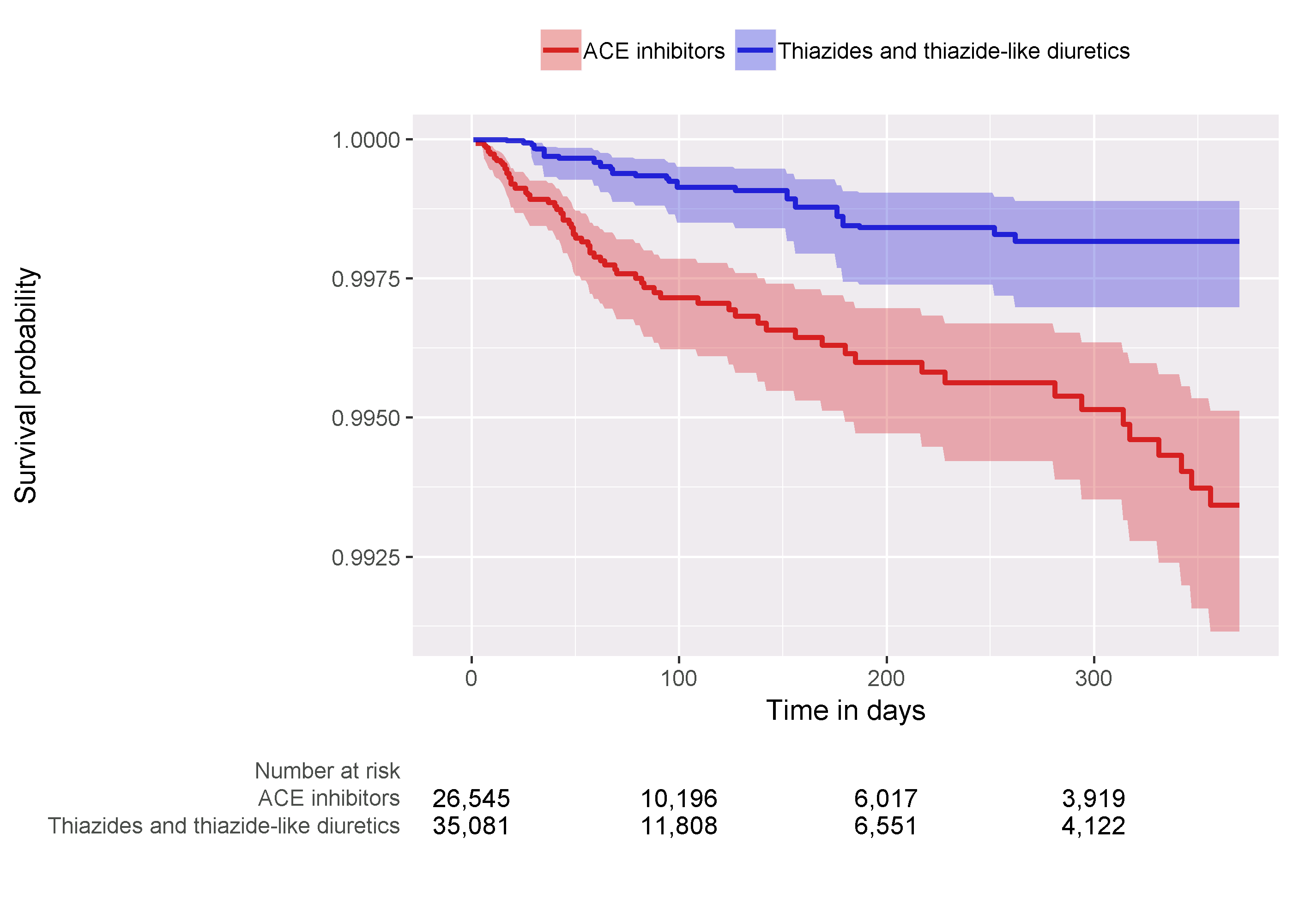
Figure 12.22: Kaplan-Meier plot.
12.9.5 Effect Size Estimate
We observe a hazard ratio of 4.32 (95% confidence interval: 2.45 - 8.08) for angioedema, which tells us that ACEi appears to increase the risk of angioedema compared to THZ. Similarly, we observe a hazard ratio of 1.13 (95% confidence interval: 0.59 - 2.18) for AMI, suggesting little or no effect for AMI. Our diagnostics, as reviewed earlier, give no reason for doubt. However, ultimately the quality of this evidence, and whether we choose to trust it, depends on many factors that are not covered by the study diagnostics as described in Chapter 14.
12.10 Summary
Population-level estimation aims to infer causal effects from observational data.
The counterfactual, what would have happened if the subject had received an alternative exposure or no exposure, cannot be observed.
Different designs aim to construct the counterfactual in different ways.
The various designs as implemented in the OHDSI Methods Library provide diagnostics to evaluate whether the assumptions for creating an appropriate counterfactual have been met.
12.11 Exercises
Prerequisites
For these exercises we assume R, R-Studio and Java have been installed as described in Section 8.4.5. Also required are the SqlRender, DatabaseConnector, Eunomia and CohortMethod packages, which can be installed using:
install.packages(c("SqlRender", "DatabaseConnector", "remotes"))
remotes::install_github("ohdsi/Eunomia", ref = "v1.0.0")
remotes::install_github("ohdsi/CohortMethod")
The Eunomia package provides a simulated dataset in the CDM that will run inside your local R session. The connection details can be obtained using:
The CDM database schema is “main”. These exercises also make use of several cohorts. The createCohorts function in the Eunomia package will create these in the COHORT table:
Problem Definition
What is the risk of gastrointestinal (GI) bleed in new users of celecoxib compared to new users of diclofenac?
The celecoxib new-user cohort has COHORT_DEFINITION_ID = 1. The diclofenac new-user cohort has COHORT_DEFINITION_ID = 2. The GI bleed cohort has COHORT_DEFINITION_ID = 3. The ingredient concept IDs for celecoxib and diclofenac are 1118084 and 1124300, respectively. Time-at-risk starts on day of treatment initiation, and stops at the end of observation (a so-called intent-to-treat analysis).
Exercise 12.1 Using the CohortMethod R package, use the default set of covariates and extract the CohortMethodData from the CDM. Create the summary of the CohortMethodData.
Exercise 12.2 Create a study population using the createStudyPopulation function, requiring a 180-day washout period, excluding people who had a prior outcome, and removing people that appear in both cohorts. Did we lose people?
Exercise 12.3 Fit a Cox proportional hazards model without using any adjustments. What could go wrong if you do this?
Exercise 12.4 Fit a propensity model. Are the two groups comparable?
Exercise 12.5 Perform PS stratification using 5 strata. Is covariate balance achieved?
Exercise 12.6 Fit a Cox proportional hazards model using the PS strata. Why is the result different from the unadjusted model?
Suggested answers can be found in Appendix E.8.
References
Austin, Peter C. 2011. “Optimal Caliper Widths for Propensity-Score Matching When Estimating Differences in Means and Differences in Proportions in Observational Studies.” Pharmaceutical Statistics 10 (2): 150–61.
Farrington, C. P. 1995. “Relative incidence estimation from case series for vaccine safety evaluation.” Biometrics 51 (1): 228–35.
Farrington, C. P., Karim Anaya-Izquierdo, Heather J. Whitaker, Mounia N. Hocine, Ian Douglas, and Liam Smeeth. 2011. “Self-Controlled Case Series Analysis with Event-Dependent Observation Periods.” Journal of the American Statistical Association 106 (494): 417–26. https://doi.org/10.1198/jasa.2011.ap10108.
Hernan, M. A., S. Hernandez-Diaz, M. M. Werler, and A. A. Mitchell. 2002. “Causal knowledge as a prerequisite for confounding evaluation: an application to birth defects epidemiology.” Am. J. Epidemiol. 155 (2): 176–84.
Hernan, M. A., and J. M. Robins. 2016. “Using Big Data to Emulate a Target Trial When a Randomized Trial Is Not Available.” Am. J. Epidemiol. 183 (8): 758–64.
Maclure, M. 1991. “The case-crossover design: a method for studying transient effects on the risk of acute events.” Am. J. Epidemiol. 133 (2): 144–53.
Magid, D. J., S. M. Shetterly, K. L. Margolis, H. M. Tavel, P. J. O’Connor, J. V. Selby, and P. M. Ho. 2010. “Comparative effectiveness of angiotensin-converting enzyme inhibitors versus beta-blockers as second-line therapy for hypertension.” Circ Cardiovasc Qual Outcomes 3 (5): 453–58.
Powers, B. J., R. R. Coeytaux, R. J. Dolor, V. Hasselblad, U. D. Patel, W. S. Yancy, R. N. Gray, R. J. Irvine, A. S. Kendrick, and G. D. Sanders. 2012. “Updated report on comparative effectiveness of ACE inhibitors, ARBs, and direct renin inhibitors for patients with essential hypertension: much more data, little new information.” J Gen Intern Med 27 (6): 716–29.
Rassen, J. A., A. A. Shelat, J. Myers, R. J. Glynn, K. J. Rothman, and S. Schneeweiss. 2012. “One-to-many propensity score matching in cohort studies.” Pharmacoepidemiol Drug Saf 21 Suppl 2 (May): 69–80.
Rosenbaum, P., and D. Rubin. 1983. “The Central Role of the Propensity Score in Observational Studies for Causal Effects.” Biometrika 70 (April): 41–55. https://doi.org/10.1093/biomet/70.1.41.
Rubin, Donald B. 2001. “Using Propensity Scores to Help Design Observational Studies: Application to the Tobacco Litigation.” Health Services and Outcomes Research Methodology 2 (3-4): 169–88.
Ryan, P. B., M. J. Schuemie, and D. Madigan. 2013. “Empirical performance of a self-controlled cohort method: lessons for developing a risk identification and analysis system.” Drug Saf 36 Suppl 1 (October): 95–106.
Sabroe, R. A., and A. K. Black. 1997. “Angiotensin-converting enzyme (ACE) inhibitors and angio-oedema.” Br. J. Dermatol. 136 (2): 153–58.
Schneeweiss, S. 2018. “Automated data-adaptive analytics for electronic healthcare data to study causal treatment effects.” Clin Epidemiol 10: 771–88.
Simpson, S. E., D. Madigan, I. Zorych, M. J. Schuemie, P. B. Ryan, and M. A. Suchard. 2013. “Multiple self-controlled case series for large-scale longitudinal observational databases.” Biometrics 69 (4): 893–902.
Suchard, M. A., S. E. Simpson, Ivan Zorych, P. B. Ryan, and David Madigan. 2013. “Massive Parallelization of Serial Inference Algorithms for a Complex Generalized Linear Model.” ACM Trans. Model. Comput. Simul. 23 (1): 10:1–10:17. https://doi.org/10.1145/2414416.2414791.
Suissa, S. 1995. “The case-time-control design.” Epidemiology 6 (3): 248–53.
Tian, Y., M. J. Schuemie, and M. A. Suchard. 2018. “Evaluating large-scale propensity score performance through real-world and synthetic data experiments.” Int J Epidemiol 47 (6): 2005–14.
Toh, S., M. E. Reichman, M. Houstoun, M. Ross Southworth, X. Ding, A. F. Hernandez, M. Levenson, et al. 2012. “Comparative risk for angioedema associated with the use of drugs that target the renin-angiotensin-aldosterone system.” Arch. Intern. Med. 172 (20): 1582–9.
Vandenbroucke, J. P., and N. Pearce. 2012. “Case-control studies: basic concepts.” Int J Epidemiol 41 (5): 1480–9.
Walker, Alexander M, Amanda R Patrick, Michael S Lauer, Mark C Hornbrook, Matthew G Marin, Richard Platt, Véronique L Roger, Paul Stang, and Sebastian Schneeweiss. 2013. “A Tool for Assessing the Feasibility of Comparative Effectiveness Research.” Comp Eff Res 3: 11–20.
Whelton, P. K., R. M. Carey, W. S. Aronow, D. E. Casey, K. J. Collins, C. Dennison Himmelfarb, S. M. DePalma, et al. 2018. “2017 ACC/AHA/AAPA/ABC/ACPM/AGS/APhA/ASH/ASPC/NMA/PCNA Guideline for the Prevention, Detection, Evaluation, and Management of High Blood Pressure in Adults: Executive Summary: A Report of the American College of Cardiology/American Heart Association Task Force on Clinical Practice Guidelines.” Circulation 138 (17): e426–e483.
Whitaker, H. J., C. P. Farrington, B. Spiessens, and P. Musonda. 2006. “Tutorial in biostatistics: the self-controlled case series method.” Stat Med 25 (10): 1768–97.
Wickham, Hadley. 2015. R Packages. 1st ed. O’Reilly Media, Inc.
Zaman, M. A., S. Oparil, and D. A. Calhoun. 2002. “Drugs targeting the renin-angiotensin-aldosterone system.” Nat Rev Drug Discov 1 (8): 621–36.