Chapter 13 Patient-Level Prediction
Chapter leads: Peter Rijnbeek & Jenna Reps
Clinical decision making is a complicated task in which the clinician has to infer a diagnosis or treatment pathway based on the available medical history of the patient and the current clinical guidelines. Clinical prediction models have been developed to support this decision-making process and are used in clinical practice in a wide spectrum of specialties. These models predict a diagnostic or prognostic outcome based on a combination of patient characteristics, e.g. demographic information, disease history, and treatment history.
The number of publications describing clinical prediction models has increased strongly over the last 10 years. Most currently-used models are estimated using small datasets and consider only a small set of patient characteristics. This low sample size, and thus low statistical power, forces the data analyst to make strong modelling assumptions. The selection of the limited set of patient characteristics is strongly guided by the expert knowledge at hand. This contrasts sharply with the reality of modern medicine wherein patients generate a rich digital trail, which is well beyond the power of any medical practitioner to fully assimilate. Presently, health care is generating a huge amount of patient-specific information stored in Electronic Health Records (EHRs). This includes structured data in the form of diagnosis, medication, laboratory test results, and unstructured data contained in clinical narratives. It is unknown how much predictive accuracy can be gained by leveraging the large amount of data originating from the complete EHR of a patient.
Advances in machine learning for large dataset analysis have led to increased interest in applying patient-level prediction on this type of data. However, many published efforts in patient-level prediction do not follow the model development guidelines, fail to perform extensive external validation, or provide insufficient model details which limits the ability of independent researchers to reproduce the models and perform external validation. This makes it hard to fairly evaluate the predictive performance of the models and reduces the likelihood of the model being used appropriately in clinical practice. To improve standards, several papers have been written detailing guidelines for best practices in developing and reporting prediction models. For example, the Transparent Reporting of a multivariable prediction model for Individual Prognosis Or Diagnosis (TRIPOD) statement56 provides clear recommendations for reporting prediction model development and validation and addresses some of the concerns related to transparency.
Massive-scale, patient-specific predictive modeling has become reality due to OHDSI, where the Common Data Model (CDM) allows for uniform and transparent analysis at an unprecedented scale. The growing network of databases standardized to the CDM enables external validation of models in different healthcare settings on a global scale. We believe this provides immediate opportunity to serve large communities of patients who are in most need of improved quality of care. Such models can inform truly personalized medical care, leading hopefully to sharply improved patient outcomes.
In this chapter we describe OHDSI’s standardized framework for patient-level prediction, (Reps et al. 2018) and discuss the PatientLevelPrediction R package that implements established best practices for development and validation. We start with providing the necessary theory behind the development and evaluation of patient-level prediction and provide a high-level overview of the implemented machine learning algorithms. We then discuss an example prediction problem and provide step-by-step guidance on its definition and implementation using ATLAS or custom R code. Finally, we discuss the use of Shiny applications for the dissemination of study results.
13.1 The Prediction Problem
Figure 13.1 illustrates the prediction problem we address. Among a population at risk, we aim to predict which patients at a defined moment in time (t = 0) will experience some outcome during a time-at-risk. Prediction is done using only information about the patients in an observation window prior to that moment in time.
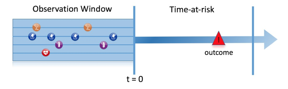
Figure 13.1: The prediction problem.
As shown in Table 13.1, to define a prediction problem we have to define t=0 by a target cohort, the outcome we like to predict by an outcome cohort, and the time-at-risk. We define the standard prediction question as:
Among [target cohort definition], who will go on to have [outcome cohort definition] within [time-at-risk period]?
Furthermore, we have to make design choices for the model we like to develop, and determine the observational datasets to perform internal and external validation.
| Choice | Description |
|---|---|
| Target cohort | How do we define the cohort of persons for whom we wish to predict? |
| Outcome cohort | How do we define the outcome we want to predict? |
| Time-at-risk | In which time window relative to t=0 do we want to make the prediction? |
| Model | What algorithms do we want to use, and which potential predictor variables do we include? |
This conceptual framework works for all types of prediction problems, for example:
- Disease onset and progression
- Structure: Among patients who are newly diagnosed with [a disease], who will go on to have [another disease or complication] within [time horizon from diagnosis]?
- Example: Among newly diagnosed atrial fibrillation patients, who will go on to have ischemic stroke in the next three years?
- Treatment choice
- Structure: Among patients with [indicated disease] who are treated with either [treatment 1] or [treatment 2], which patients were treated with [treatment 1]?
- Example: Among patients with atrial fibrillation who took either warfarin or rivaroxaban, which patients get warfarin? (e.g. for a propensity model)
- Treatment response
- Structure: Among new users of [a treatment], who will experience [some effect] in [time window] ?
- Example: Which patients with diabetes who start on metformin stay on metformin for three years?
- Treatment safety
- Structure: Among new users of [a treatment], who will experience [adverse event] in [time window]?
- Example: Among new users of warfarin, who will have a gastrointestinal bleed in one year?
- Treatment adherence
- Structure: Among new users of [a treatment], who will achieve [adherence metric] at [time window]?
- Example: Which patients with diabetes who start on metformin achieve >=80% proportion of days covered at one year?
13.2 Data Extraction
When creating a predictive model we use a process known as supervised learning — a form of machine learning — that infers the relationship between the covariates and the outcome status based on a labelled set of examples. Therefore, we need methods to extract the covariates from the CDM for the persons in the target cohort and we need to obtain their outcome labels.
The covariates (also referred to as “predictors”, “features” or “independent variables”) describe the characteristics of the patients. Covariates can include age, gender, presence of specific conditions and exposure codes in a patient’s record, etc. Covariates are typically constructed using the FeatureExtraction package, described in more detail in Chapter 11. For prediction we can only use data prior to (and on) the date the person enters the target cohort. This date we will call the index date.
We also need to obtain the outcome status (also referred to as the “labels” or “classes”) of all the patients during the time-at-risk. If the outcome occurs within the time-at-risk, the outcome status is defined as “positive.”
13.2.1 Data Extraction Example
Table 13.2 shows an example COHORT table with two cohorts. The cohort with cohort definition ID 1 is the target cohort (e.g. “people recently diagnosed with atrial fibrillation”). Cohort definition ID 2 defines the outcome cohort (e.g. “stroke”).
| COHORT_DEFINITION_ID | SUBJECT_ID | COHORT_START_DATE |
|---|---|---|
| 1 | 1 | 2000-06-01 |
| 1 | 2 | 2001-06-01 |
| 2 | 2 | 2001-07-01 |
Table 13.3 provides an example CONDITION_OCCURRENCE table. Concept ID 320128 refers to “Essential hypertension.”
| PERSON_ID | CONDITION_CONCEPT_ID | CONDITION_START_DATE |
|---|---|---|
| 1 | 320128 | 2000-10-01 |
| 2 | 320128 | 2001-05-01 |
Based on this example data, and assuming the time at risk is the year following the index date (the target cohort start date), we can construct the covariates and the outcome status. A covariate indicating “Essential hypertension in the year prior” will have the value 0 (not present) for person ID 1 (the condition occurred after the index date), and the value 1 (present) for person ID 2. Similarly, the outcome status will be 0 for person ID 1 (this person had no entry in the outcome cohort), and 1 for person ID 2 (the outcome occurred within a year following the index date).
13.2.2 Negative vs Missing
Observational healthcare data rarely reflects whether a value is negative or missing. In the prior example, we simply observed the person with ID 1 had no essential hypertension occurrence prior to the index date. This could be because the condition was not present (negative) at that time, or because it was not recorded (missing). It is important to realize that the machine learning algorithm cannot distinguish between the negative and missing and will simply assess the predictive value in the available data.
13.3 Fitting the Model
When fitting a prediction model we are trying to learn the relationship between the covariates and the observed outcome status from labelled examples. Suppose we only have two covariates, systolic and diastolic blood pressure, then we can represent each patient as a plot in two dimensional space as shown in Figure 13.2. In this figure the shape of the data point corresponds to the patient’s outcome status (e.g. stroke).
A supervised learning model will try to find a decision boundary that optimally separates the two outcome classes. Different supervised learning techniques lead to different decision boundaries and there are often hyper-parameters that can impact the complexity of the decision boundary.
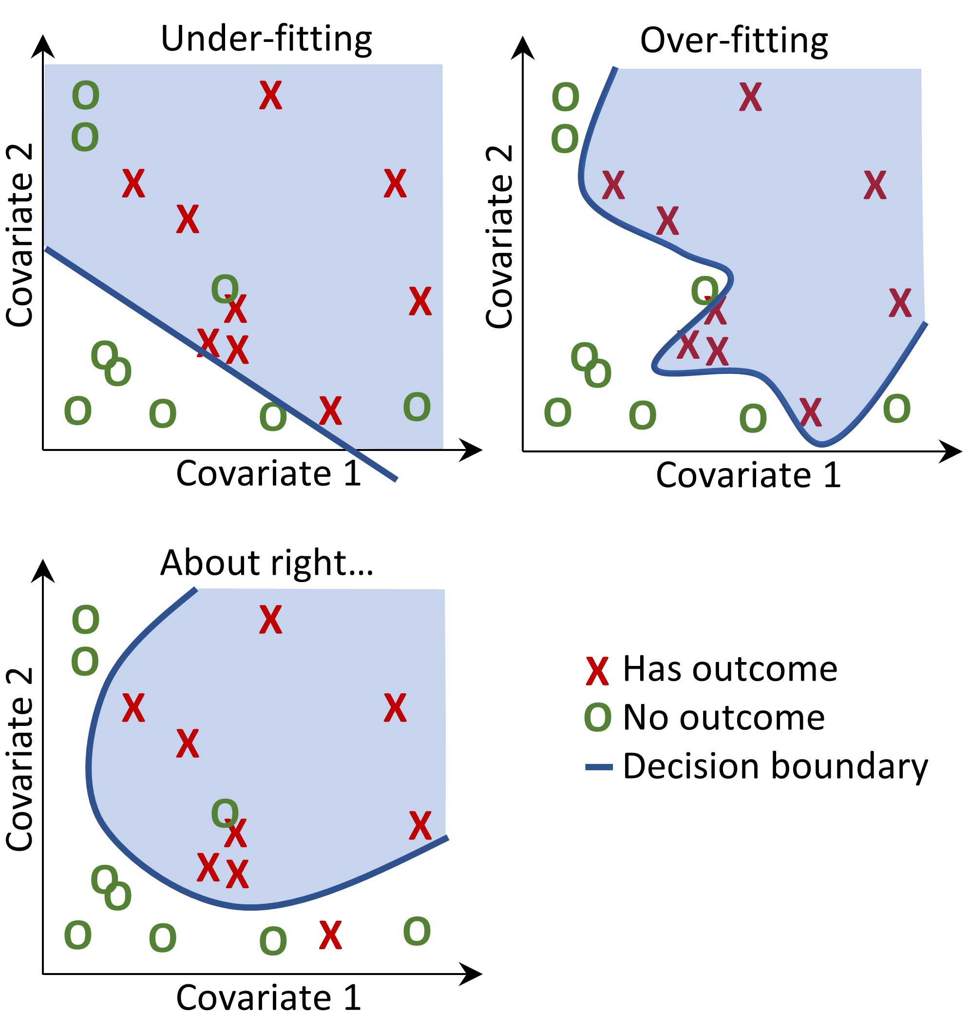
Figure 13.2: Decision boundary.
In Figure 13.2 we can see three different decision boundaries. The boundaries are used to infer the outcome status of any new data point. If a new data point falls into the shaded area then the model will predict “has outcome”, otherwise it will predict “no outcome”. Ideally a decision boundary should perfectly partition the two classes. However, there is a risk that too complex models “overfit” to the data. This can negatively impact the generalizability of the model to unseen data. For example, if the data contains noise, with mislabeled or incorrectly positioned data points, we would not want to fit our model to that noise. We therefore may prefer to define a decision boundary that does not perfectly discriminate in our training data but captures the “real” complexity. Techniques such as regularization aim to maximize model performance while minimizing complexity.
Each supervised learning algorithm has a different way to learn the decision boundary and it is not straightforward which algorithm will work best on your data. As the No Free Lunch theorem states not one algorithm is always going to outperform the others on all prediction problems. Therefore, we recommend trying multiple supervised learning algorithms with various hyper-parameter settings when developing patient-level prediction models.
The following algorithms are available in the PatientLevelPrediction package:
13.3.1 Regularized Logistic Regression
LASSO (least absolute shrinkage and selection operator) logistic regression belongs to the family of generalized linear models, where a linear combination of the variables is learned and finally a logistic function maps the linear combination to a value between 0 and 1. The LASSO regularization adds a cost based on model complexity to the objective function when training the model. This cost is the sum of the absolute values of the linear combination of the coefficients. The model automatically performs feature selection by minimizing this cost. We use the Cyclops (Cyclic coordinate descent for logistic, Poisson and survival analysis) package to perform large-scale regularized logistic regression.
| Parameter | Description | Typical values |
|---|---|---|
| Starting variance | The starting variance of the prior distribution. | 0.1 |
Note that the variance is optimized by maximizing the out-of-sample likelihood in a cross-validation, so the starting variance has little impact on the performance of the resulting model. However, picking a starting variance that is too far from the optimal value may lead to long fitting time.
13.3.2 Gradient Boosting Machines
Gradient boosting machines is a boosting ensemble technique and in our framework it combines multiple decision trees. Boosting works by iteratively adding decision trees but adds more weight to the data-points that are misclassified by prior decision trees in the cost function when training the next tree. We use Extreme Gradient Boosting, which is an efficient implementation of the gradient boosting framework implemented in the xgboost R package available from CRAN.
| Parameter | Description | Typical values |
|---|---|---|
| earlyStopRound | Stopping after rounds without improvement | 25 |
| learningRate | The boosting learn rate | 0.005,0.01,0.1 |
| maxDepth | Max levels in a tree | 4,6,17 |
| minRows | Min data points in a node | 2 |
| ntrees | Number of trees | 100,1000 |
13.3.3 Random Forest
Random forest is a bagging ensemble technique that combines multiple decision trees. The idea behind bagging is to reduce the likelihood of overfitting by using weak classifiers and combining them into a strong classifier. Random forest accomplishes this by training multiple decision trees but only using a subset of the variables in each tree and the subset of variables differ between trees. Our package uses the sklearn implementation of Random Forest in Python.
| Parameter | Description | Typical values |
|---|---|---|
| maxDepth | Max levels in a tree | 4,10,17 |
| mtries | Number of features in each tree | -1 = square root of total features,5,20 |
| ntrees | Number of trees | 500 |
13.3.4 K-Nearest Neighbors
K-nearest neighbors (KNN) is an algorithm that uses some distance metric to find the K closest labelled data-points to a new unlabeled data-point. The prediction of the new data-points is then the most prevalent class of the K-nearest labelled data-points. There is a sharing limitation of KNN, as the model requires labelled data to perform the prediction on new data, and it is often not possible to share this data across data sites. We included the BigKnn package developed in OHDSI which is a large scale KNN classifier.
| Parameter | Description | Typical values |
|---|---|---|
| k | Number of neighbors | 1000 |
13.3.5 Naive Bayes
The Naive Bayes algorithm applies the Bayes theorem with the naive assumption of conditional independence between every pair of features given the value of the class variable. Based on the likelihood the data belongs to a class and the prior distribution of the class, a posterior distribution is obtained. Naive Bayes has no hyper-parameters.
13.3.6 AdaBoost
AdaBoost is a boosting ensemble technique. Boosting works by iteratively adding classifiers but adds more weight to the data-points that are misclassified by prior classifiers in the cost function when training the next classifier. We use the sklearn AdaboostClassifier implementation in Python.
| Parameter | Description | Typical values |
|---|---|---|
| nEstimators | The maximum number of estimators at which boosting is terminated | 4 |
| learningRate | Learning rate shrinks the contribution of each classifier by learning_rate. There is a trade-off between learningRate and nEstimators | 1 |
13.3.7 Decision Tree
A decision tree is a classifier that partitions the variable space using individual tests selected using a greedy approach. It aims to find partitions that have the highest information gain to separate the classes. The decision tree can easily overfit by enabling a large number of partitions (tree depth) and often needs some regularization (e.g., pruning or specifying hyper-parameters that limit the complexity of the model). We use the sklearn DecisionTreeClassifier implementation in Python.
| Parameter | Description | Typical values |
|---|---|---|
| classWeight | “Balance” or “None” | None |
| maxDepth | The maximum depth of the tree | 10 |
| minImpuritySplit | Threshold for early stopping in tree growth. A node will split if its impurity is above the threshold, otherwise it is a leaf | 10^-7 |
| minSamplesLeaf | The minimum number of samples per leaf | 10 |
| minSamplesSplit | The minimum samples per split | 2 |
13.3.8 Multilayer Perceptron
Multilayer perceptrons are neural networks that contain multiple layers of nodes that weight their inputs using a non-linear function. The first layer is the input layer, the last layer is the output layer, and in between are the hidden layers. Neural networks are generally trained using back-propagation, meaning the training input is propagated forward through the network to produce an output, the error between the output and the outcome status is computed, and this error is propagated backwards through the network to update the linear function weights.
| Parameter | Description | Typical values |
|---|---|---|
| alpha | The l2 regularization | 0.00001 |
| size | The number of hidden nodes | 4 |
13.3.9 Deep Learning
Deep learning such as deep nets, convolutional neural networks or recurrent neural networks are similar to Multilayer Perceptrons but have multiple hidden layers that aim to learn latent representations useful for prediction. In a separate vignette in the PatientLevelPrediction package we describe these models and hyper-parameters in more detail.
13.3.10 Other Algorithms
Other algorithms can be added to the patient-level prediction framework. This is out-of-scope for this chapter. Details can be found in the “Adding Custom Patient-Level Prediction Algorithms” vignette in the PatientLevelPrediction package.
13.4 Evaluating Prediction Models
13.4.1 Evaluation Types
We can evaluate a prediction model by measuring the agreement between the model’s prediction and observed outcome status, which means we need data where the outcome status is known.
We distinguish between
- Internal validation: Using different sets of data extracted from the same database to develop and evaluate the model.
- External validation: Developing the model in one database, and evaluating in another database.
There are two ways to perform internal validation:
- A holdout set approach splits the labelled data into two independent sets: a train set and a test set (the hold out set). The train set is used to learn the model and the test set is used to evaluate it. We can simply divide our patients randomly into a train and test set, or we may choose to:
- Split the data based on time (temporal validation), for example training on data before a specific date, and evaluating on data after that date. This may inform us on whether our model generalizes to different time periods.
- Split the data based on geographic location (spatial validation).
- Cross validation is useful when the data are limited. The data is split into \(n\) equally-sized sets, where \(n\) needs to be prespecified (e.g. \(n=10\)). For each of these sets a model is trained on all data except the data in that set and used to generate predictions for the hold-out set. In this way, all data is used once to evaluate the model-building algorithm. In the patient-level prediction framework we use cross validation to pick the optimal hyper-parameters.
External validation aims to assess model performance on data from another database, i.e. outside of the settings it was developed in. This measure of model transportability is important because we want to apply our models not only on the database it was trained on. Different databases may represent different patient populations, different healthcare systems and different data-capture processes. We believe that the external validation of prediction models on a large set of databases is a crucial step in model acceptance and implementation in clinical practice.
13.4.2 Performance Metrics
Threshold Measures
A prediction model assigns a value between 0 and 1 for each patient corresponding to the risk of the patient having the outcome during the time at risk. A value of 0 means 0% risk, a value of 0.5 means 50% risk and a value of 1 means 100% risk. Common metrics such as accuracy, sensitivity, specificity, positive predictive value can be calculated by first specifying a threshold that is used to classify patients as having the outcome or not during the time at risk. For example, given Table 13.11, if we set the threshold as 0.5, patients 1, 3, 7 and 10 have a predicted risk greater than or equal to the threshold of 0.5 so they would be predicted to have the outcome. All other patients had a predicted risk less than 0.5, so they would be predicted to not have the outcome.
| Patient ID | Predicted risk | Predicted class at 0.5 threshold | Has outcome during time-at-risk | Type |
|---|---|---|---|---|
| 1 | 0.8 | 1 | 1 | TP |
| 2 | 0.1 | 0 | 0 | TN |
| 3 | 0.7 | 1 | 0 | FP |
| 4 | 0 | 0 | 0 | TN |
| 5 | 0.05 | 0 | 0 | TN |
| 6 | 0.1 | 0 | 0 | TN |
| 7 | 0.9 | 1 | 1 | TP |
| 8 | 0.2 | 0 | 1 | FN |
| 9 | 0.3 | 0 | 0 | TN |
| 10 | 0.5 | 1 | 0 | FP |
If a patient is predicted to have the outcome and has the outcome (during the time-at-risk) then this is called a true positive (TP). If a patient is predicted to have the outcome but does not have the outcome then this is called a false positive (FP). If a patient is predicted to not have the outcome and does not have the outcome then this is called a true negative (TN). Finally, if a patient is predicted to not have the outcome but does have the outcome then this is called a false negative (FN).
The following threshold-based metrics can be calculated:
- accuracy: \((TP+TN)/(TP+TN+FP+FN)\)
- sensitivity: \(TP/(TP+FN)\)
- specificity: \(TN/(TN+FP)\)
- positive predictive value: \(TP/(TP+FP)\)
Note that these values can either decrease or increase if the threshold is lowered. Lowering the threshold of a classifier may increase the denominator by increasing the number of results returned. If the threshold was previously set too high, the new results may all be true positives, which will increase positive predictive value. If the previous threshold was about right or too low, further lowering the threshold will introduce false positives, decreasing positive predictive value. For sensitivity the denominator does not depend on the classifier threshold (\(TP+FN\) is a constant). This means that lowering the classifier threshold may increase sensitivity by increasing the number of true positive results. It is also possible that lowering the threshold may leave sensitivity unchanged, while the positive predictive value fluctuates.
Discrimination
Discrimination is the ability to assign a higher risk to patients who will experience the outcome during the time at risk. The Receiver Operating Characteristics (ROC) curve is created by plotting 1 – specificity on the x-axis and sensitivity on the y-axis at all possible thresholds. An example ROC plot is presented later in this chapter in Figure 13.17. The area under the receiver operating characteristic curve (AUC) gives an overall measure of discrimination where a value of 0.5 corresponds to randomly assigning the risk and a value of 1 means perfect discrimination. Most published prediction models obtain AUCs between 0.6-0.8.
The AUC provides a way to determine how different the predicted risk distributions are between the patients who experience the outcome during the time at risk and those who do not. If the AUC is high, then the distributions will be mostly disjointed, whereas when there is a lot of overlap, the AUC will be closer to 0.5, as shown in Figure 13.3.
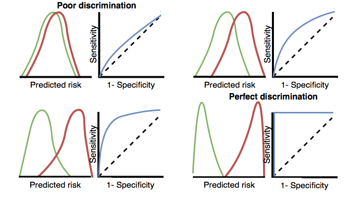
Figure 13.3: How the ROC plots are linked to discrimination. If the two classes have similar distributions of predicted risk, the ROC will be close to the diagonal, with AUC close to 0.5.
For rare outcomes even a model with a high AUC may not be practical, because for every positive above a given threshold there could also be many negatives (i.e. the positive predictive value will be low). Depending on the severity of the outcome and cost (health risk and/or monetary) of some intervention, a high false positive rate may be unwanted. When the outcome is rare another measure known as the area under the precision-recall curve (AUPRC) is therefore recommended. The AUPRC is the area under the line generated by plotting the sensitivity on the x-axis (also known as the recall) and the positive predictive value (also known as the precision) on the y-axis.
Calibration
Calibration is the ability of the model to assign the correct risk. For example, if the model assigned one hundred patients a risk of 10% then ten of the patients should experience the outcome during the time at risk. If the model assigned 100 patients a risk of 80% then eighty of the patients should experience the outcome during the time at risk. The calibration is generally calculated by partitioning the patients into deciles based on the predicted risk and in each group calculating the mean predicted risk and the fraction of the patients who experienced the outcome during the time at risk. We then plot these ten points (predicted risk on the y-axis and observed risk on the x-axis) and see whether they fall on the x = y line, indicating the model is well calibrated. An example calibration plot is presented later in this chapter in Figure 13.18. We also fit a linear model using the points to calculate the intercept (which should be close to zero) and the gradient (which should be close to one). If the gradient is greater than one then the model is assigning a higher risk than the true risk and if the gradient is less than one the model is assigning a lower risk than the true risk. Note that we also implemented Smooth Calibration Curves in our R-package to better capture the non-linear relationship between predicted and observed risk.
13.5 Designing a Patient-Level Prediction Study
In this section we will demonstrate how to design a prediction study. The first step is to clearly define the prediction problem. Interestingly, in many published papers the prediction problem is poorly defined, for example it is unclear how the index date (start of the target cohort) is defined. A poorly defined prediction problem does not allow for external validation by others, let alone implementation in clinical practice. In the patient-level prediction framework we enforce proper specification of the prediction problem by requiring the key choices defined in Table 13.1 to be explicitly defined. Here we will walk through this process using a “treatment safety” type prediction problem as an example.
13.5.1 Problem Definition
Angioedema is a well-known side-effect of ACE inhibitors, and the incidence of angioedema reported in the labeling for ACE inhibitors is in the range of 0.1% to 0.7%. (Byrd, Adam, and Brown 2006) Monitoring patients for this adverse effect is important, because although angioedema is rare, it may be life-threatening, leading to respiratory arrest and death. (Norman et al. 2013) Further, if angioedema is not initially recognized, it may lead to extensive and expensive workups before it is identified as a cause. (Norman et al. 2013; Thompson and Frable 1993) Other than the higher risk among African-American patients, there are no known predisposing factors for the development of ACE inhibitor related angioedema. (Byrd, Adam, and Brown 2006) Most reactions occur within the first week or month of initial therapy and often within hours of the initial dose. (Cicardi et al. 2004) However, some cases may occur years after therapy has begun. (O’Mara and O’Mara 1996) No diagnostic test is available that specifically identifies those at risk. If we could identify those at risk, doctors could act, for example by discontinuing the ACE inhibitor in favor of another hypertension drug.
We will apply the patient-level prediction framework to observational healthcare data to address the following patient-level prediction question:
Among patients who have just started on an ACE inhibitor for the first time, who will experience angioedema in the following year?
13.5.2 Study Population Definition
The final study population in which we will develop our model is often a subset of the target cohort, because we may for example apply criteria that are dependent on the outcome, or we want to perform sensitivity analyses with sub-populations of the target cohort. For this we have to answer the following questions:
What is the minimum amount of observation time we require before the start of the target cohort? This choice could depend on the available patient time in the training data, but also on the time we expect to be available in the data sources we want to apply the model on in the future. The longer the minimum observation time, the more baseline history time is available for each person to use for feature extraction, but the fewer patients will qualify for analysis. Moreover, there could be clinical reasons to choose a short or longer look-back period. For our example, we will use a 365-day prior history as look-back period (washout period).
Can patients enter the target cohort multiple times? In the target cohort definition, a person may qualify for the cohort multiple times during different spans of time, for example if they had different episodes of a disease or separate periods of exposure to a medical product. The cohort definition does not necessarily apply a restriction to only let the patients enter once, but in the context of a particular patient-level prediction problem we may want to restrict the cohort to the first qualifying episode. In our example, a person can only enter the target cohort once since our criteria was based on first use of an ACE inhibitor.
Do we allow persons to enter the cohort if they experienced the outcome before? Do we allow persons to enter the target cohort if they experienced the outcome before qualifying for the target cohort? Depending on the particular patient-level prediction problem, there may be a desire to predict incident first occurrence of an outcome, in which case patients who have previously experienced the outcome are not at risk for having a first occurrence and therefore should be excluded from the target cohort. In other circumstances, there may be a desire to predict prevalent episodes, whereby patients with prior outcomes can be included in the analysis and the prior outcome itself can be a predictor of future outcomes. For our prediction example, we will choose not to include those with prior angioedema.
How do we define the period in which we will predict our outcome relative to the target cohort start? We have to make two decisions to answer this question. First, does the time-at-risk window start at the date of the start of the target cohort or later? Arguments to make it start later could be that we want to avoid outcomes that were entered late in the record that actually occurred before the start of the target cohort or we want to leave a gap where interventions to prevent the outcome could theoretically be implemented. Second, we need to define the time-at-risk by setting the risk window end, as some specification of days offset relative to the target cohort start or end dates. For our problem we will predict in a time-at-risk window starting 1 day after the start of the target cohort up to 365 days later.
Do we require a minimum amount of time-at-risk? We have to decide if we want to include patients that did not experience the outcome but did leave the database earlier than the end of our time-at-risk period. These patients may experience the outcome when we no longer observe them. For our prediction problem we decide to answer this question with “yes,” requiring a minimum time-at-risk for that reason. Furthermore, we have to decide if this constraint also applies to persons who experienced the outcome or we will include all persons with the outcome irrespective of their total time at risk. For example, if the outcome is death, then persons with the outcome are likely censored before the full time-at-risk period is complete.
13.5.3 Model Development Settings
To develop the prediction model we have to decide which algorithm(s) we like to train. We see the selection of the best algorithm for a certain prediction problem as an empirical question, i.e. we prefer to let the data speak for itself and try different approaches to find the best one. In our framework we have therefore implemented many algorithms as described in Section 13.3, and allow others to be added. In this example, to keep things simple, we select just one algorithm: Gradient Boosting Machines.
Furthermore, we have to decide on the covariates that we will use to train our model. In our example, we like to add gender, age, all conditions, drugs and drug groups, and visit counts. We will look for these clinical events in the year before and any time prior to the index date.
13.5.4 Model Evaluation
Finally, we have to define how we will evaluate our model. For simplicity, we here choose internal validation. We have to decide how we divide our dataset in a training and test dataset and how we assign patients to these two sets. Here we will use a typical 75% - 25% split. Note that for very large datasets we could use more data for training.
13.5.5 Study Summary
We have now completely defined our study as shown in Table 13.12.
| Choice | Value |
|---|---|
| Target cohort | Patients who have just started on an ACE inhibitor for the first time. Patients are excluded if they have less than 365 days of prior observation time or have prior angioedema. |
| Outcome cohort | Angioedema. |
| Time-at-risk | 1 day until 365 days from cohort start. We will require at least 364 days at risk. |
| Model | Gradient Boosting Machine with hyper-parameters ntree: 5000, max depth: 4 or 7 or 10 and learning rate: 0.001 or 0.01 or 0.1 or 0.9. Covariates will include gender, age, conditions, drugs, drug groups, and visit count. Data split: 75% train - 25% test, randomly assigned by person. |
13.6 Implementing the Study in ATLAS
The interface for designing a prediction study can be opened by clicking on the  button in the left hand side ATLAS menu. Create a new prediction study. Make sure to give the study an easy-to-recognize name. The study design can be saved at any time by clicking the
  button.
In the Prediction design function, there are four sections: Prediction Problem Settings, Analysis Settings, Execution Settings, and Training Settings. Here we discuss each section:
13.6.1 Prediction Problem Settings
Here we select the target population cohorts and outcome cohorts for the analysis. A prediction model will be developed for all combinations of the target population cohorts and the outcome cohorts. For example, if we specify two target populations and two outcomes, we have specified four prediction problems.
To select a target population cohort we need to have previously defined it in ATLAS. Instantiating cohorts is described in Chapter 10. The Appendix provides the full definitions of the target (Appendix B.1) and outcome (Appendix B.4) cohorts used in this example. To add a target population to the cohort, click on the “Add Target Cohort” button. Adding outcome cohorts similarly works by clicking the “Add Outcome Cohort” button. When done, the dialog should look like Figure 13.4.
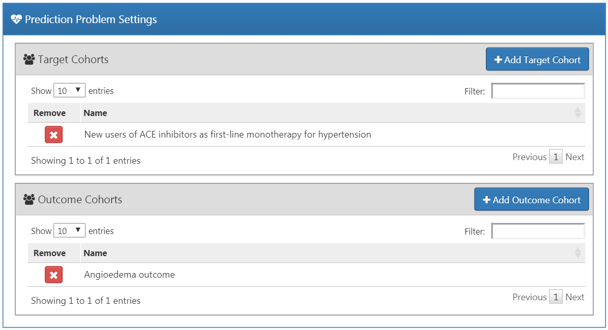
Figure 13.4: Prediction problem settings.
13.6.2 Analysis Settings
The analysis settings enable selection of the supervised learning algorithm, the covariates and population settings.
Model Settings
We can pick one or more supervised learning algorithms for model development. To add a supervised learning algorithm click on the “Add Model Settings” button. A dropdown containing all the models currently supported in the ATLAS interface will appear. We can select the supervised learning model we want to include in the study by clicking on the name in the dropdown menu. This will then show a view for that specific model, allowing the selection of the hyper-parameter values. If multiple values are provided, a grid search is performed across all possible combinations of values to select the optimal combination using cross-validation.
For our example we select gradient boosting machines, and set the hyper-parameters as specified in Figure 13.5.
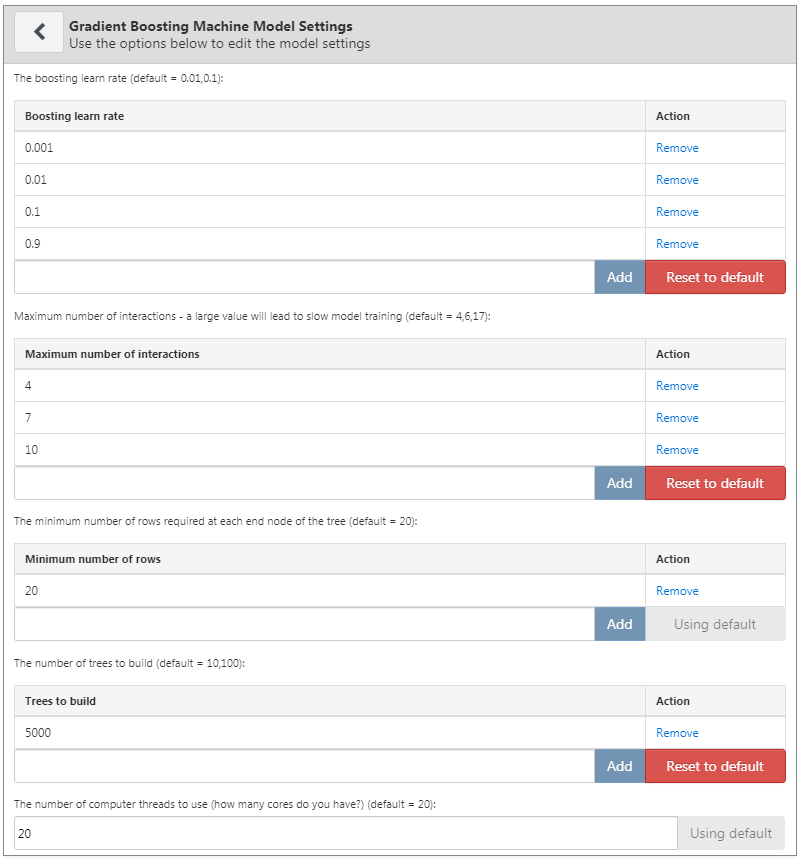
Figure 13.5: Gradient boosting machine settings
Covariate Settings
We have defined a set of standard covariates that can be extracted from the observational data in the CDM format. In the covariate settings view, it is possible to select which of the standard covariates to include. We can define different types of covariate settings, and each model will be created separately with each specified covariate setting.
To add a covariate setting into the study, click on the “Add Covariate Settings”. This will open the covariate setting view.
The first part of the covariate settings view is the exclude/include option. Covariates are generally constructed for any concept. However, we may want to include or exclude specific concepts, for example if a concept is linked to the target cohort definition. To only include certain concepts, create a concept set in ATLAS and then under the “What concepts do you want to include in baseline covariates in the patient-level prediction model? (Leave blank if you want to include everything)” select the concept set by clicking on  . We can automatically add all descendant concepts to the concepts in the concept set by answering “yes” to the question “Should descendant concepts be added to the list of included concepts?” The same process can be repeated for the question “What concepts do you want to exclude in baseline covariates in the patient-level prediction model? (Leave blank if you want to include everything)”, allowing covariates corresponding to the selected concepts to be removed. The final option “A comma delimited list of covariate IDs that should be restricted to” enables us to add a set of covariate IDs (rather than concept IDs) comma separated that will only be included in the model. This option is for advanced users only. Once done, the inclusion and exclusion settings should look like Figure 13.6.
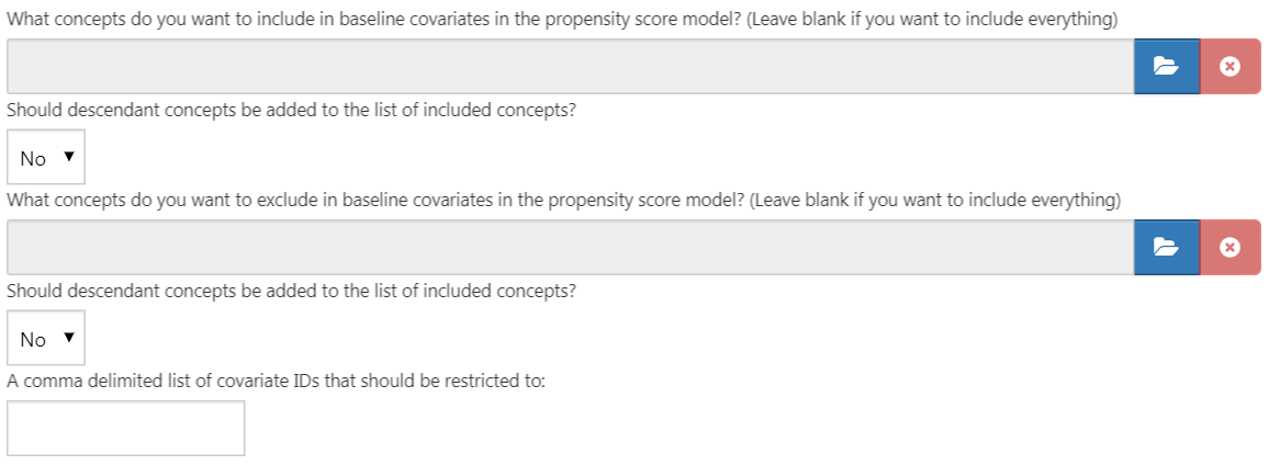
Figure 13.6: Covariate inclusion and exclusion settings.
The next section enables the selection of non-time bound variables.
- Gender: a binary variable indicating male or female gender
- Age: a continuous variable corresponding to age in years
- Age group: binary variables for every 5 years of age (0-4, 5-9, 10-14, …, 95+)
- Race: a binary variable for each race, 1 means the patient has that race recorded, 0 otherwise
- Ethnicity: a binary variable for each ethnicity, 1 means the patient has that ethnicity recorded, 0 otherwise
- Index year: a binary variable for each cohort start date year, 1 means that was the patients cohort start date year, 0 otherwise. It often does not make sense to include index year, since we would like to apply our model to the future.
- Index month - a binary variable for each cohort start date month, 1 means that was the patient’s cohort start date month, 0 otherwise
- Prior observation time: [Not recommended for prediction] a continuous variable corresponding to how long in days the patient was in the database prior to the cohort start date
- Post observation time: [Not recommended for prediction] a continuous variable corresponding to how long in days the patient was in the database post cohort start date
- Time in cohort: a continuous variable corresponding to how long in days the patient was in the cohort (cohort end date minus cohort start date)
- Index year and month: [Not recommended for prediction] a binary variable for each cohort start date year and month combination, 1 means that was the patients cohort start date year and month, 0 otherwise
Once done, this section should look like Figure 13.7.
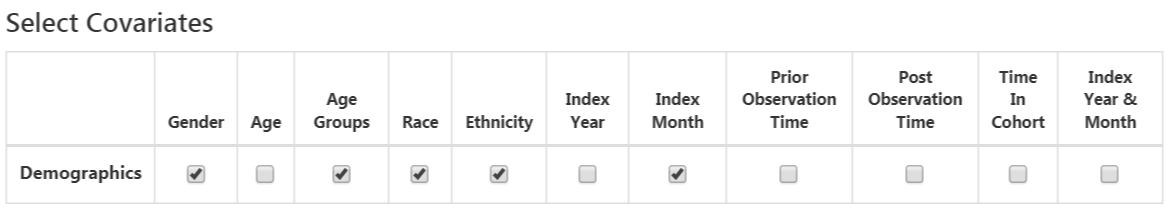
Figure 13.7: Select covariates.
The standard covariates enable three flexible time intervals for the covariates:
- end days: when to end the time intervals relative to the cohort start date [default is 0]
- long term [default -365 days to end days prior to cohort start date]
- medium term [default -180 days to end days prior to cohort start date]
- short term [default -30 days to end days prior to cohort start date]
Once done, this section should look like Figure 13.8.
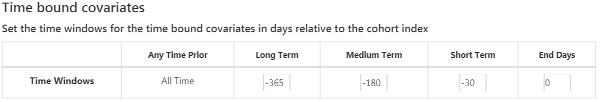
Figure 13.8: Time bound covariates.
The next option is the covariates extracted from the era tables:
- Condition: Construct covariates for each condition concept ID and time interval selected and if a patient has the concept ID with an era (i.e., the condition starts or ends during the time interval or starts before and ends after the time interval) during the specified time interval prior to the cohort start date in the condition era table, the covariate value is 1, otherwise 0.
- Condition group: Construct covariates for each condition concept ID and time interval selected and if a patient has the concept ID or any descendant concept ID with an era during the specified time interval prior to the cohort start date in the condition era table, the covariate value is 1, otherwise 0.
- Drug: Construct covariates for each drug concept ID and time interval selected and if a patient has the concept ID with an era during the specified time interval prior to the cohort start date in the drug era table, the covariate value is 1, otherwise 0.
- Drug group: Construct covariates for each drug concept ID and time interval selected and if a patient has the concept ID or any descendant concept ID with an era during the specified time interval prior to the cohort start date in the drug era table, the covariate value is 1, otherwise 0.
Overlapping time interval setting means that the drug or condition era should start prior to the cohort start date and end after the cohort start date, so it overlaps with the cohort start date. The era start option restricts to finding condition or drug eras that start during the time interval selected.
Once done, this section should look like Figure 13.9.
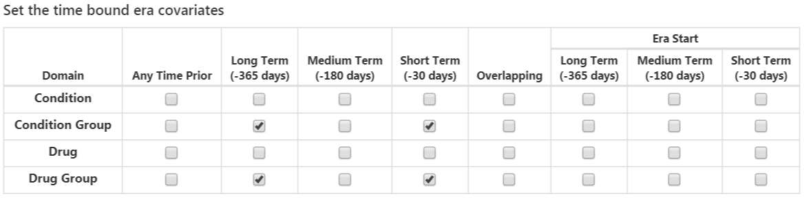
Figure 13.9: Time bound era covariates.
The next option selects covariates corresponding to concept IDs in each domain for the various time intervals:
- Condition: Construct covariates for each condition concept ID and time interval selected and if a patient has the concept ID recorded during the specified time interval prior to the cohort start date in the condition occurrence table, the covariate value is 1, otherwise 0.
- Condition Primary Inpatient: One binary covariate per condition observed as a primary diagnosis in an inpatient setting in the condition_occurrence table.
- Drug: Construct covariates for each drug concept ID and time interval selected and if a patient has the concept ID recorded during the specified time interval prior to the cohort start date in the drug exposure table, the covariate value is 1, otherwise 0.
- Procedure: Construct covariates for each procedure concept ID and time interval selected and if a patient has the concept ID recorded during the specified time interval prior to the cohort start date in the procedure occurrence table, the covariate value is 1, otherwise 0.
- Measurement: Construct covariates for each measurement concept ID and time interval selected and if a patient has the concept ID recorded during the specified time interval prior to the cohort start date in the measurement table, the covariate value is 1, otherwise 0.
- Measurement Value: Construct covariates for each measurement concept ID with a value and time interval selected and if a patient has the concept ID recorded during the specified time interval prior to the cohort start date in the measurement table, the covariate value is the measurement value, otherwise 0.
- Measurement range group: Binary covariates indicating whether measurements are below, within, or above normal range.
- Observation: Construct covariates for each observation concept ID and time interval selected and if a patient has the concept ID recorded during the specified time interval prior to the cohort start date in the observation table, the covariate value is 1, otherwise 0.
- Device: Construct covariates for each device concept ID and time interval selected and if a patient has the concept ID recorded during the specified time interval prior to the cohort start date in the device table, the covariate value is 1, otherwise 0.
- Visit Count: Construct covariates for each visit and time interval selected and count the number of visits recorded during the time interval as the covariate value.
- Visit Concept Count: Construct covariates for each visit, domain and time interval selected and count the number of records per domain recorded during the visit type and time interval as the covariate value.
The distinct count option counts the number of distinct concept IDs per domain and time interval.
Once done, this section should look like Figure 13.10.
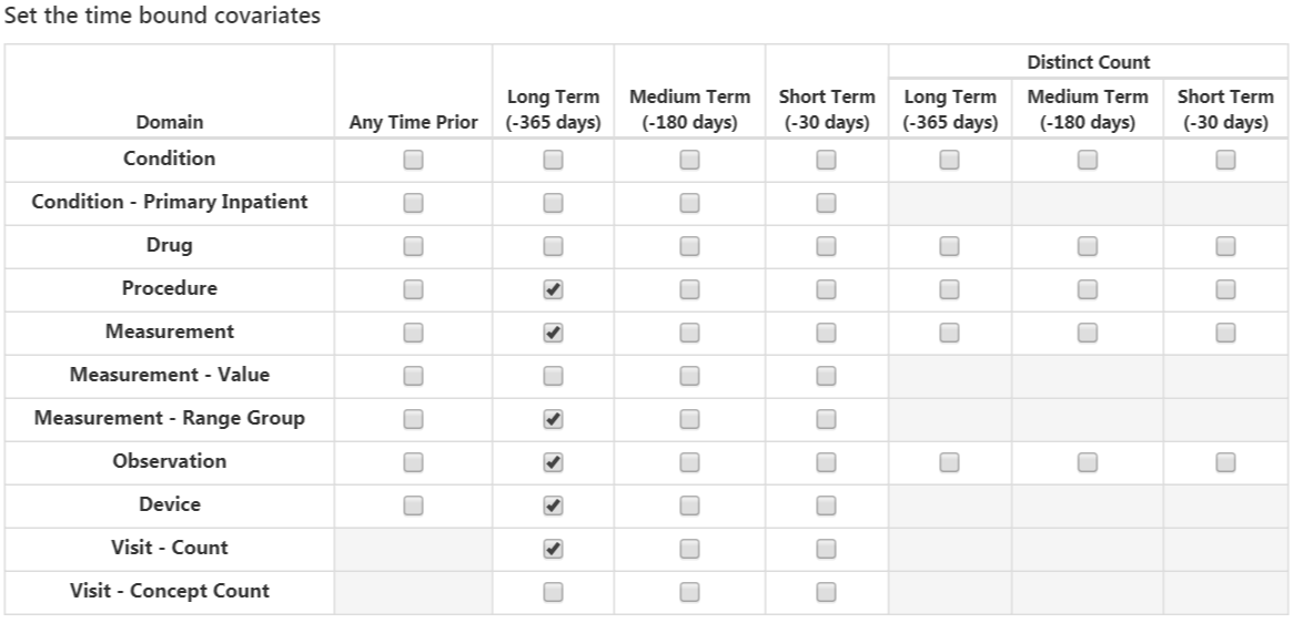
Figure 13.10: Time bound covariates.
The final option is whether to include commonly used risk scores as covariates. Once done, the risk score settings should look like Figure 13.11.
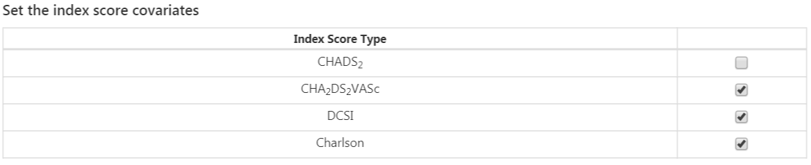
Figure 13.11: Risk score covariate settings.
Population Settings
The population settings is where addition inclusion criteria can be applied to the target population and is also where the time-at-risk is defined. To add a population setting into the study, click on the “Add Population Settings” button. This will open up the population setting view.
The first set of options enable the user to specify the time-at-risk period. This is the time interval where we look to see whether the outcome of interest occurs. If a patient has the outcome during the time-at-risk period then we will classify them as “Has outcome”, otherwise they are classified as “No outcome”. “Define the time-at-risk window start, relative to target cohort entry:” defines the start of the time-at-risk, relative to the target cohort start or end date. Similarly, “Define the time-at-risk window end:” defines the end of the time-at-risk.
“Minimum lookback period applied to target cohort” specifies the minimum baseline period, the minimum number of days prior to the cohort start date that a patient is continuously observed. The default is 365 days. Expanding the minimum look-back will give a more complete picture of a patient (as they must have been observed for longer) but will filter patients who do not have the minimum number of days prior observation.
If “Should subjects without time at risk be removed?” is set to yes, then a value for “Minimum time at risk:” is also required. This allows removing people who are lost to follow-up (i.e. that have left the database during the time-at-risk period). For example, if the time-at-risk period was 1 day from cohort start until 365 days from cohort start, then the full time-at-risk interval is 364 days (365-1). If we only want to include patients who are observed the whole interval, then we set the minimum time at risk to be 364. If we are happy as long as people are in the time-at-risk for the first 100 days, then we select minimum time at risk to be 100. In this case as the time-at-risk start is 1 day from the cohort start, a patient will be included if they remain in the database for at least 101 days from the cohort start date. If we set “Should subjects without time at risk be removed?” to ‘No’, then this will keep all patients, even those who drop out from the database during the time-at-risk.
The option “Include people with outcomes who are not observed for the whole at risk period?” is related to the previous option. If set to “yes”, then people who experience the outcome during the time-at-risk are always kept, even if they are not observed for the specified minimum amount of time.
The option “Should only the first exposure per subject be included?” is only useful if our target cohort contains patients multiple times with different cohort start dates. In this situation, picking “yes” will result in only keeping the earliest target cohort date per patient in the analysis. Otherwise a patient can be in the dataset multiple times.
Setting “Remove patients who have observed the outcome prior to cohort entry?” to “yes” will remove patients who have the outcome prior to the time-at-risk start date, so the model is for patients who have never experienced the outcome before. If “no” is selected, then patients could have had the outcome prior. Often, having the outcome prior is very predictive of having the outcome during the time-at-risk.
Once done, the population settings dialog should look like Figure 13.12.
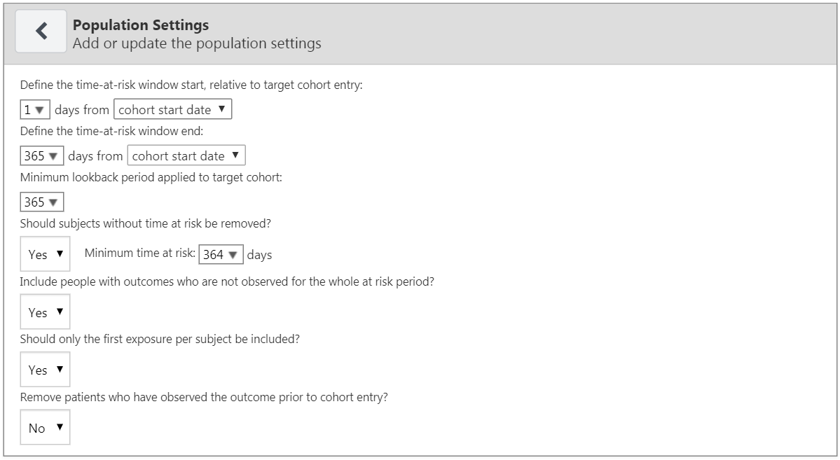
Figure 13.12: Population settings.
Now that we are finished with the Analysis Settings, the entire dialog should look like Figure 13.13.
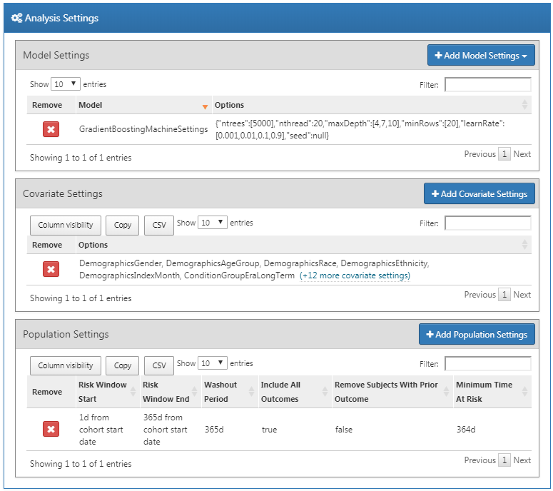
Figure 13.13: Analysis settings.
13.6.3 Execution Settings
There are three options:
- “Perform sampling”: here we choose whether to perform sampling (default = “no”). If set to “yes”, another option will appear: “How many patients to use for a subset?”, where the sample size can be specified. Sampling can be an efficient means to determine if a model for a large population (e.g. 10 million patients) will be predictive by creating and testing the model with a sample of patients. For example, if the AUC is close to 0.5 in the sample, we might abandon the model.
- “Minimum covariate occurrence: If a covariate occurs in a fraction of the target population less than this value, it will be removed:”: here we choose the minimum covariate occurrence (default = 0.001). A minimum threshold value for covariate occurrence is necessary to remove rare events that are not representative of the overall population.
- “Normalize covariate”: here we choose whether to normalize covariates (default = “yes”). Normalization of the covariates is usually necessary for successful implementation of a LASSO model.
For our example we make the choices shown in Figure 13.14.
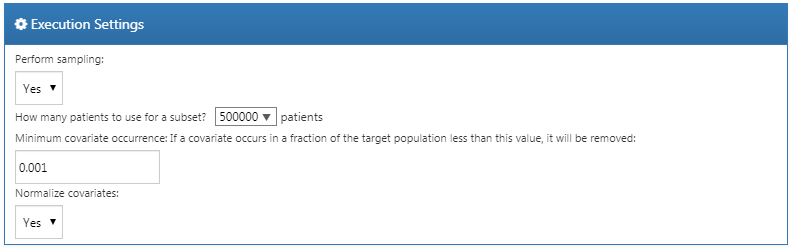
Figure 13.14: Execution settings.
13.6.4 Training Settings
There are four options:
- “Specify how to split the test/train set:” Select whether to differentiate the train/test data by person (stratified by outcome) or by time (older data to train the model, later data to evaluate the model).
- “Percentage of the data to be used as the test set (0-100%)”: Select the percentage of data to be used as test data (default = 25%).
- “The number of folds used in the cross validation”: Select the number of folds for cross-validation used to select the optimal hyper-parameter (default = 3).
- “The seed used to split the test/train set when using a person type testSplit (optional):”: Select the random seed used to split the train/test set when using a person type test split.
For our example we make the choices shown in Figure 13.15.
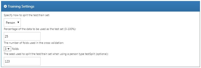
Figure 13.15: Training settings.
13.6.5 Importing and Exporting a Study
To export a study, click on the “Export” tab under “Utilities.” ATLAS will produce JSON that can be directly copied and pasted into a file that contains all of the data, such as the study name, cohort definitions, models selected, covariates, settings, needed to run the study.
To import a study, click on the “Import” tab under “Utilities.” Paste the contents of a patient-level prediction study JSON into this window, then click on the Import button below the other tab buttons. Note that this will overwrite all previous settings for that study, so this is typically done using a new, empty study design.
13.6.6 Downloading the Study Package
Click on the “Review & Download” tab under “Utilities.” In the “Download Study Package” section, enter a descriptive name for the R package, noting that any illegal characters in R will automatically be removed from the file name by ATLAS. Click on  to download the R package to a local folder.
13.6.7 Running the Study
To run the R package requires having R, RStudio, and Java installed as described in Section 8.4.5. Also required is the PatientLevelPrediction package, which can be installed in R using:
Some of the machine learning algorithms require additional software to be installed. For a full description of how to install the PatientLevelPrediction package, see the “Patient-Level Prediction Installation Guide” vignette.
To use the study R package we recommend using R Studio. If you are running R Studio locally, unzip the file generated by ATLAS, and double click the .Rproj file to open it in R Studio. If you are running R Studio on an R studio server, click  to upload and unzip the file, then click on the .Rproj file to open the project.
Once you have opened the project in R Studio, you can open the README file, and follow the instructions. Make sure to change all file paths to existing paths on your system.
13.7 Implementing the Study in R
An alternative to implementing our study design using ATLAS is to write the study code ourselves in R. We can make use of the functions provided in the PatientLevelPrediction package. The package enables data extraction, model building, and model evaluation using data from databases that are translated into the OMOP CDM.
13.7.1 Cohort Instantiation
We first need to instantiate the target and outcome cohorts. Instantiating cohorts is described in Chapter 10. The Appendix provides the full definitions of the target (Appendix B.1) and outcome (Appendix B.4) cohorts. In this example we will assume the ACE inhibitors cohort has ID 1, and the angioedema cohort has ID 2.
13.7.2 Data Extraction
We first need to tell R how to connect to the server. PatientLevelPrediction uses the DatabaseConnector package, which provides a function called createConnectionDetails. Type ?createConnectionDetails for the specific settings required for the various database management systems (DBMS). For example, one might connect to a PostgreSQL database using this code:
library(PatientLevelPrediction)
connDetails <- createConnectionDetails(dbms = "postgresql",
                                       server = "localhost/ohdsi",
                                       user = "joe",
                                       password = "supersecret")

cdmDbSchema <- "my_cdm_data"
cohortsDbSchema <- "scratch"
cohortsDbTable <- "my_cohorts"
cdmVersion <- "5"
The last four lines define the cdmDbSchema, cohortsDbSchema, and cohortsDbTable variables, as well as the CDM version. We will use these later to tell R where the data in CDM format live, where the cohorts of interest have been created, and what version CDM is used. Note that for Microsoft SQL Server, database schemas need to specify both the database and the schema, so for example cdmDbSchema <- "my_cdm_data.dbo".
First it makes sense to verify that the cohort creation has succeeded by counting the number of cohort entries:
sql <- paste("SELECT cohort_definition_id, COUNT(*) AS count",
"FROM @cohortsDbSchema.cohortsDbTable",
"GROUP BY cohort_definition_id")
conn <- connect(connDetails)
renderTranslateQuerySql(connection = conn,
                        sql = sql,
                        cohortsDbSchema = cohortsDbSchema,
                        cohortsDbTable = cohortsDbTable)
## cohort_definition_id count
## 1 1 527616
## 2 2 3201Now we can tell PatientLevelPrediction to extract all necessary data for our analysis. Covariates are extracted using the FeatureExtraction package. For more detailed information on the FeatureExtraction package see its vignettes. For our example study we decided to use these settings:
covariateSettings <- createCovariateSettings(
useDemographicsGender = TRUE,
                          useDemographicsAge = TRUE,
                          useConditionGroupEraLongTerm = TRUE,
                          useConditionGroupEraAnyTimePrior = TRUE,
                          useDrugGroupEraLongTerm = TRUE,
                          useDrugGroupEraAnyTimePrior = TRUE,
                          useVisitConceptCountLongTerm = TRUE,
                          longTermStartDays = -365,
                          endDays = -1)
The final step for extracting the data is to run the getPlpData function and input the connection details, the database schema where the cohorts are stored, the cohort definition IDs for the cohort and outcome, and the washout period which is the minimum number of days prior to cohort index date that the person must have been observed to be included into the data, and finally input the previously constructed covariate settings.
plpData <- getPlpData(connectionDetails = connDetails,
                      cdmDatabaseSchema = cdmDbSchema,
                      cohortDatabaseSchema = cohortsDbSchema,
                      cohortTable = cohortsDbSchema,
                      cohortId = 1,
                      covariateSettings = covariateSettings,
                      outcomeDatabaseSchema = cohortsDbSchema,
                      outcomeTable = cohortsDbSchema,
                      outcomeIds = 2,
                      sampleSize = 10000
)
There are many additional parameters for the getPlpData function which are all documented in the PatientLevelPrediction manual. The resulting plpData object uses the package ff to store information in a way that ensures R does not run out of memory, even when the data are large.
Creating the plpData object can take considerable computing time, and it is probably a good idea to save it for future sessions. Because plpData uses ff, we cannot use R’s regular save function. Instead, we’ll have to use the savePlpData function:
We can use the loadPlpData() function to load the data in a future session.
13.7.3 Additional Inclusion Criteria
The final study population is obtained by applying additional constraints on the two earlier defined cohorts, e.g., a minimum time at risk can be enforced (requireTimeAtRisk, minTimeAtRisk) and we can specify if this also applies to patients with the outcome (includeAllOutcomes). Here we also specify the start and end of the risk window relative to target cohort start. For example, if we like the risk window to start 30 days after the at-risk cohort start and end a year later we can set riskWindowStart = 30 and riskWindowEnd = 365. In some cases the risk window needs to start at the cohort end date. This can be achieved by setting addExposureToStart = TRUE which adds the cohort (exposure) time to the start date.
In the example below all the settings we defined for our study are imposed:
population <- createStudyPopulation(plpData = plpData,
                                    outcomeId = 2,
                                    washoutPeriod = 364,
                                    firstExposureOnly = FALSE,
                                    removeSubjectsWithPriorOutcome = TRUE,
                                    priorOutcomeLookback = 9999,
                                    riskWindowStart = 1,
                                    riskWindowEnd = 365,
                                    addExposureDaysToStart = FALSE,
                                    addExposureDaysToEnd = FALSE,
                                    minTimeAtRisk = 364,
                                    requireTimeAtRisk = TRUE,
                                    includeAllOutcomes = TRUE,
                                    verbosity = "DEBUG"
)
13.7.4 Model Development
In the set function of an algorithm the user can specify a list of eligible values for each hyper-parameter. All possible combinations of the hyper-parameters are included in a so-called grid search using cross-validation on the training set. If a user does not specify any value then the default value is used instead.
For example, if we use the following settings for the gradient boosting machine: ntrees = c(100,200), maxDepth = 4 the grid search will apply the gradient boosting machine algorithm with ntrees = 100 and maxDepth = 4 plus the default settings for other hyper-parameters and ntrees = 200 and maxDepth = 4 plus the default settings for other hyper-parameters. The hyper-parameters that lead to the best cross-validation performance will then be chosen for the final model. For our problem we choose to build a gradient boosting machine with several hyper-parameter values:
gbmModel <- setGradientBoostingMachine(ntrees = 5000,
                                       maxDepth = c(4,7,10),
                                       learnRate = c(0.001,0.01,0.1,0.9))
The runPlP function uses the population, plpData, and model settings to train and evaluate the model. We can use the testSplit (person/time) and testFraction parameters to split the data in a 75%-25% split and run the patient-level prediction pipeline:
gbmResults <- runPlp(population = population,
                     plpData = plpData,
                     modelSettings = gbmModel,
                     testSplit = 'person',
                     testFraction = 0.25,
                     nfold = 2,
                     splitSeed = 1234)
Under the hood the package will now use the R xgboost package to fit a a gradient boosting machine model using 75% of the data and will evaluate the model on the remaining 25%. A results data structure is returned containing information about the model, its performance, etc.
In the runPlp function there are several parameters to save the plpData, plpResults, plpPlots, evaluation, etc. objects which are all set to TRUE by default.
We can save the model using:
We can load the model using:
You can also save the full results structure using:
To load the full results structure use:
13.7.5 Internal Validation
Once we execute the study, the runPlp function returns the trained model and the evaluation of the model on the train/test sets. You can interactively view the results by running: viewPlp(runPlp = gbmResults). This will open a Shiny App in which we can view all performance measures created by the framework, including interactive plots (see Figure 13.16 in the section on the Shiny Application).
To generate and save all the evaluation plots to a folder run the following code:
The plots are described in more detail in Section 13.4.2.
13.7.6 External Validation
We recommend to always perform external validation, i.e. apply the final model on as much new datasets as feasible and evaluate its performance. Here we assume the data extraction has already been performed on a second database and stored in the newData folder. We load the model we previously fitted from the model folder:
# load the trained model
plpModel <- loadPlpModel("model")

#load the new plpData and create the population
plpData <- loadPlpData("newData")

population <- createStudyPopulation(plpData = plpData,
                                    outcomeId = 2,
                                    washoutPeriod = 364,
                                    firstExposureOnly = FALSE,
                                    removeSubjectsWithPriorOutcome = TRUE,
                                    priorOutcomeLookback = 9999,
                                    riskWindowStart = 1,
                                    riskWindowEnd = 365,
                                    addExposureDaysToStart = FALSE,
                                    addExposureDaysToEnd = FALSE,
                                    minTimeAtRisk = 364,
                                    requireTimeAtRisk = TRUE,
                                    includeAllOutcomes = TRUE
)

# apply the trained model on the new data
validationResults <- applyModel(population, plpData, plpModel)
To make things easier we also provide the externalValidatePlp function for performing external validation that also extracts the required data. Assuming we ran result <- runPlp(...) then we can extract the data required for the model and evaluate it on new data. Assuming the validation cohorts are in the table mainschema.dob.cohort with IDs 1 and 2 and the CDM data is in the schema cdmschema.dob:
valResult <- externalValidatePlp(
    plpResult = result,
    connectionDetails = connectionDetails,
    validationSchemaTarget = 'mainschema.dob',
    validationSchemaOutcome = 'mainschema.dob',
    validationSchemaCdm = 'cdmschema.dbo',
    databaseNames = 'new database',
    validationTableTarget = 'cohort',
    validationTableOutcome = 'cohort',
    validationIdTarget = 1,
    validationIdOutcome = 2
)
If we have multiple databases to validate the model on then we can run:
valResults <- externalValidatePlp(
    plpResult = result,
    connectionDetails = connectionDetails,
    validationSchemaTarget = list('mainschema.dob',
                                'difschema.dob',
                                'anotherschema.dob'),
    validationSchemaOutcome = list('mainschema.dob',
                                 'difschema.dob',
                                 'anotherschema.dob'),
    validationSchemaCdm = list('cdms1chema.dbo',
                             'cdm2schema.dbo',
                             'cdm3schema.dbo'),
    databaseNames = list('new database 1',
                       'new database 2',
                       'new database 3'),
    validationTableTarget = list('cohort1',
                               'cohort2',
                               'cohort3'),
    validationTableOutcome = list('cohort1',
                                'cohort2',
                                'cohort3'),
    validationIdTarget = list(1,3,5),
    validationIdOutcome = list(2,4,6)
)
13.8 Results Dissemination
13.8.1 Model Performance
Exploring the performance of a prediction model is easiest with the viewPlp function. This requires a results object as the input. If developing models in R we can use the result of runPLp as the input. If using the ATLAS-generated study package, then we need to load one of the models (in this example we will load Analysis_1):
Here “Analysis_1” corresponds to the analysis we specified earlier.
We can then launch the Shiny app by running:
The Shiny app opens with a summary of the performance metrics on the test and train sets (see Figure 13.16). The results show that the AUC on the train set was 0.78 and this dropped to 0.74 on the test set. The test set AUC is the more accurate measure. Overall, the model appears to be able to discriminate those who will develop the outcome in new users of ACE inhibitors but it slightly overfit as the performance on the train set is higher than the test set. The ROC plot is presented in Figure 13.17.
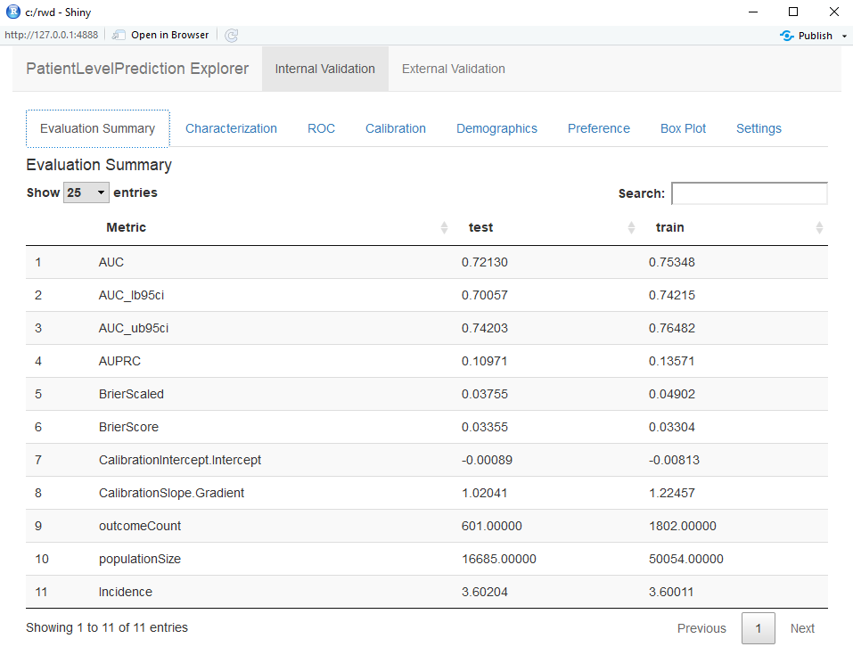
Figure 13.16: Summary evaluation statistics in the Shiny app.
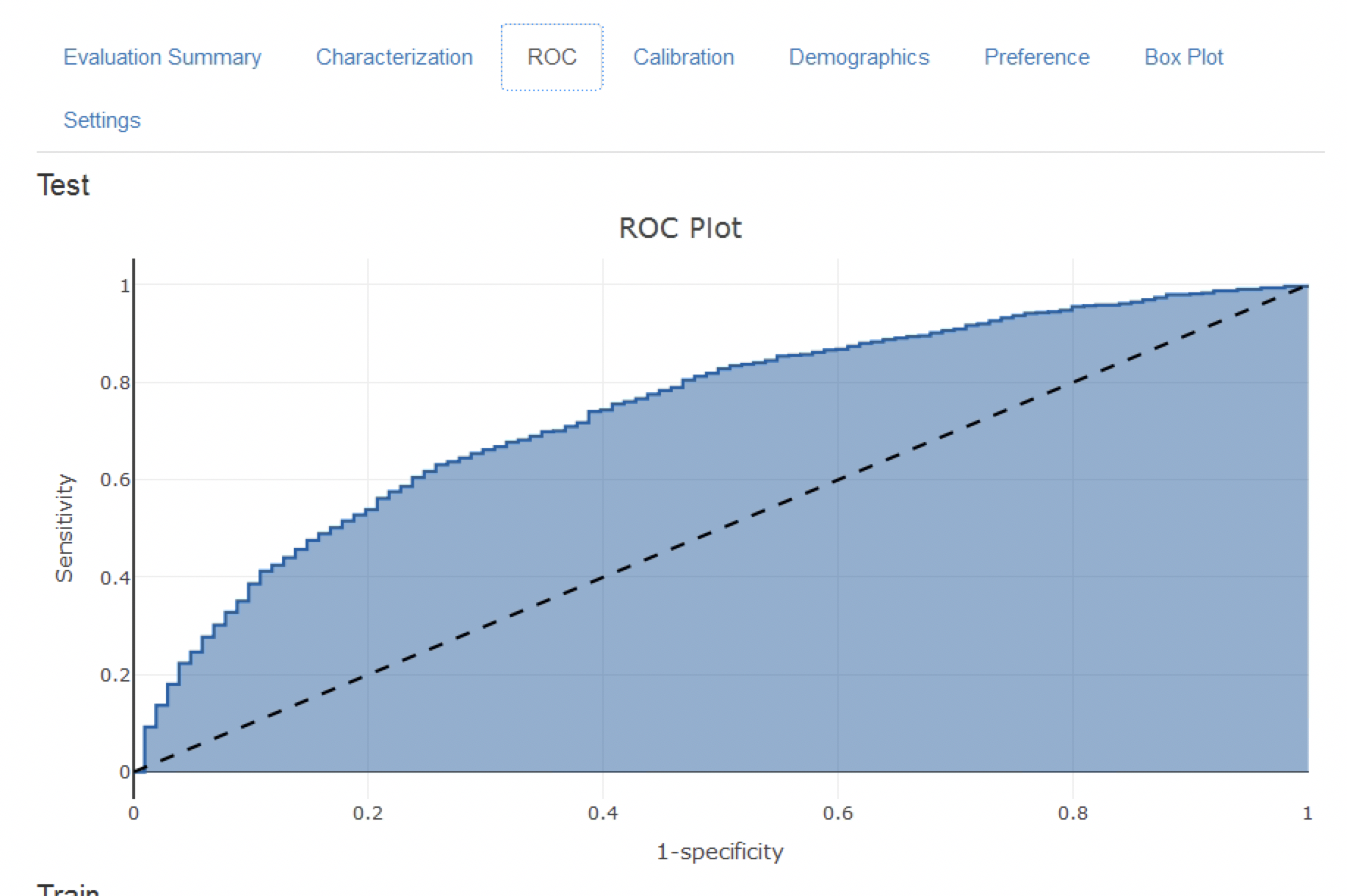
Figure 13.17: The ROC plot.
The calibration plot in Figure 13.18 shows that generally the observed risk matches the predicted risk as the dots are around the diagonal line. The demographic calibration plot in Figure 13.19 however shows that the model is not well calibrated for the younger patients, as the blue line (the predicted risk) differs from the red line (the observed risk) for those aged below 40. This may indicate we need to remove the under 40s from the target population (as the observed risk for the younger patients is nearly zero).
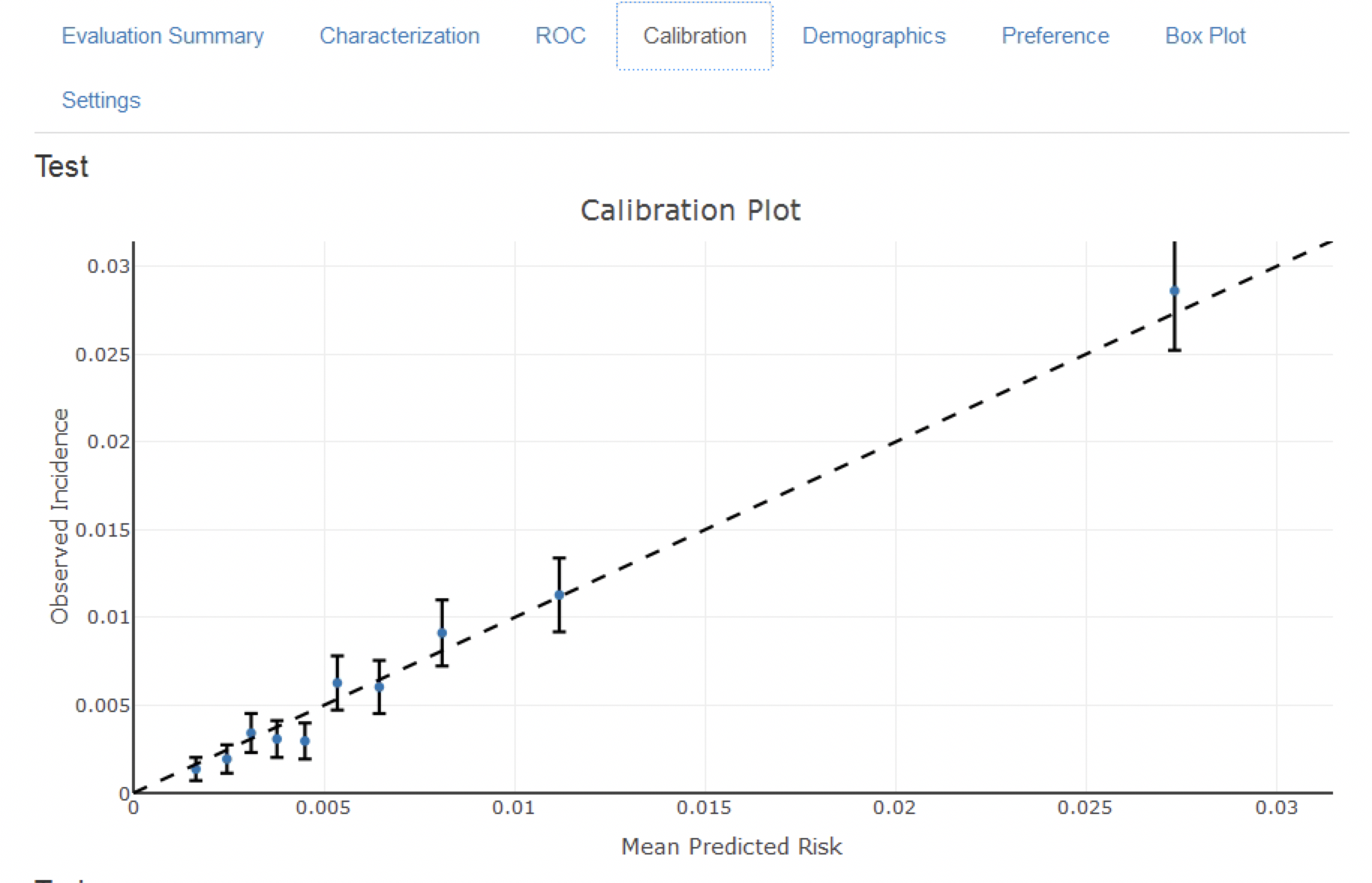
Figure 13.18: The calibration of the model
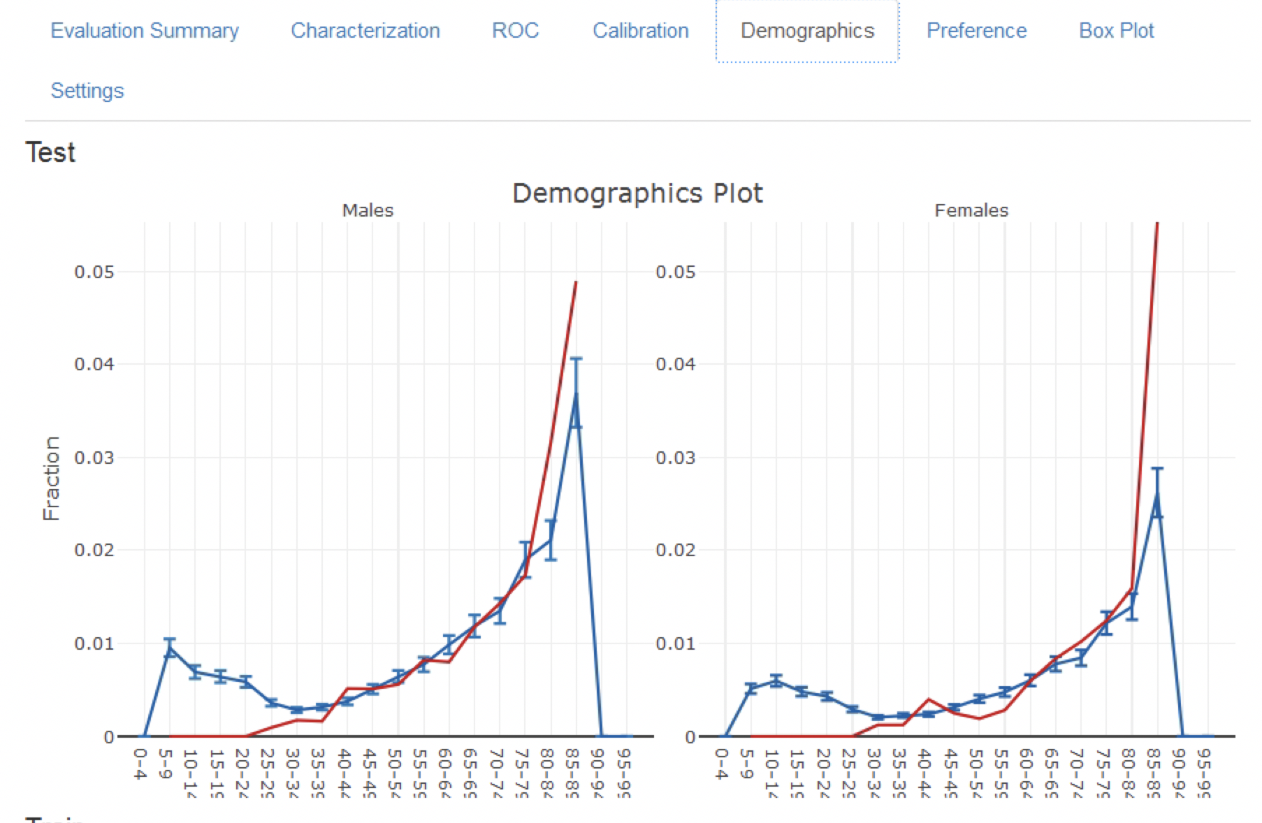
Figure 13.19: The demographic calibration of the model
Finally, the attrition plot shows the loss of patients from the labelled data based on inclusion/exclusion criteria (see Figure 13.20). The plot shows that we lost a large portion of the target population due to them not being observed for the whole time at risk (1 year follow up). Interestingly, not as many patients with the outcome lacked the complete time at risk.
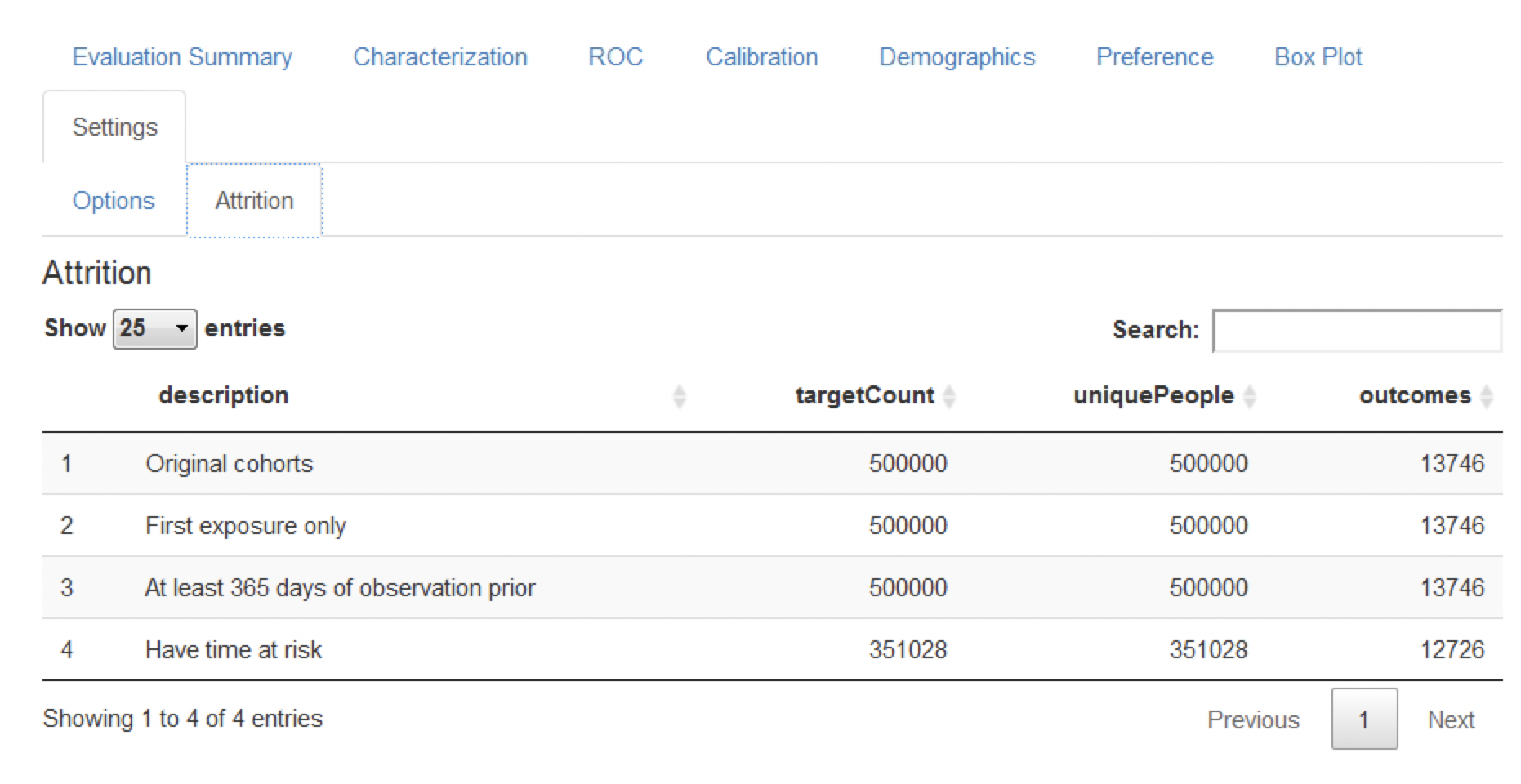
Figure 13.20: The attrition plot for the prediction problem
13.8.2 Comparing Models
The study package as generated by ATLAS allows generating and evaluating many different prediction models for different prediction problems. Therefore, specifically for the output generated by the study package an additional Shiny app has been developed for viewing multiple models. To start this app, run viewMultiplePlp(outputFolder) where outputFolder is the path containing the analysis results as specified when running the execute command (and should for example contain a sub-folder named “Analysis_1”).
Viewing the Model Summary and Settings
The interactive Shiny app will start at the summary page as shown in Figure 13.21.
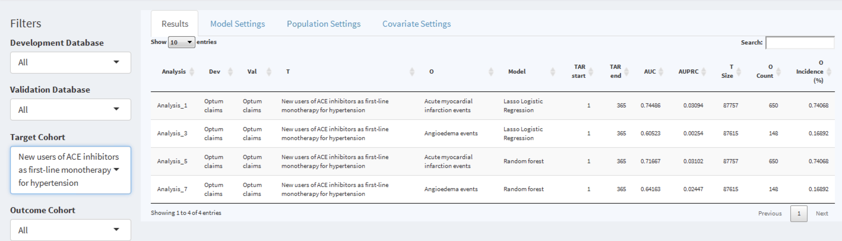
Figure 13.21: The shiny summary page containing key hold out set performance metrics for each model trained
This summary page table contains:
- basic information about the model (e.g., database information, classifier type, time-at-risk settings, target population and outcome names)
- hold out target population count and incidence of outcome
- discrimination metrics: AUC, AUPRC
To the left of the table is the filter option, where we can specify the development/validation databases to focus on, the type of model, the time at risk settings of interest and/or the cohorts of interest. For example, to pick the models corresponding to the target population “New users of ACE inhibitors as first line mono-therapy for hypertension”, select this in the Target Cohort option.
To explore a model click on the corresponding row, a selected row will be highlighted. With a row selected, we can now explore the model settings used when developing the model by clicking on the Model Settings tab:
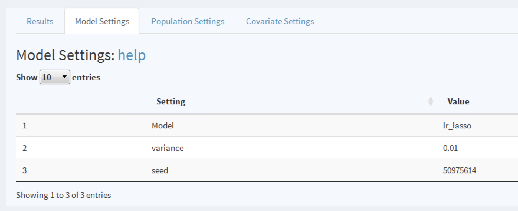
Figure 13.22: To view the model settings used when developing the model.
Similarly, we can explore the population and covariate settings used to generate the model in the other tabs.
Viewing Model Performance
Once a model row has been selected we can also view the model performance. Click on  to open the threshold performance summary shown in Figure 13.23.
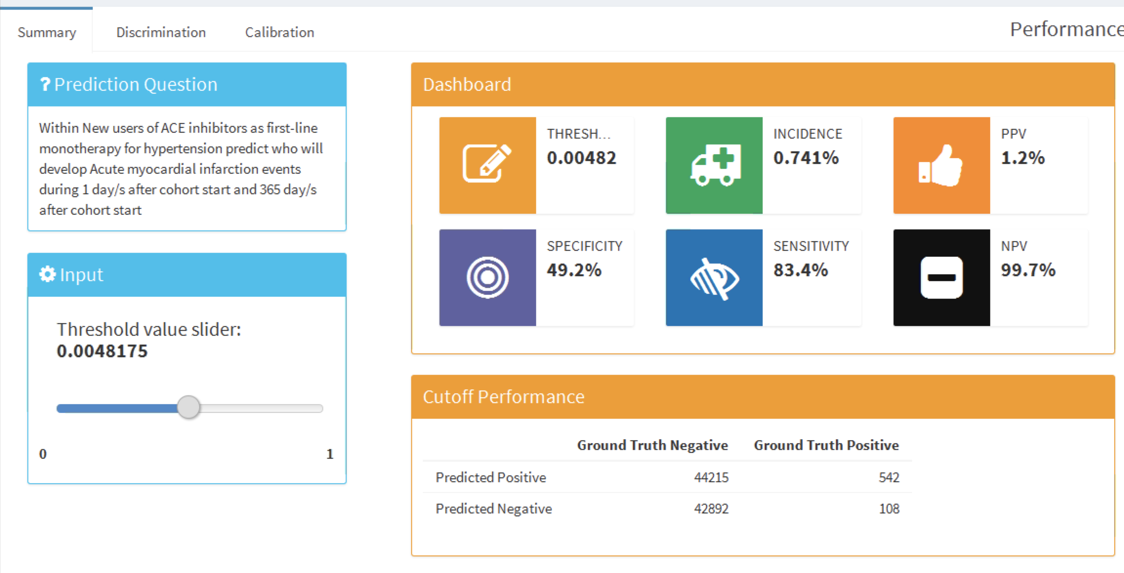
Figure 13.23: The summary performance measures at a set threshold.
This summary view shows the selected prediction question in the standard format, a threshold selector and a dashboard containing key threshold-based metrics such as positive predictive value (PPV), negative predictive value (NPV), sensitivity and specificity (see Section 13.4.2). In Figure 13.23 we see that at a threshold of 0.00482 the sensitivity is 83.4% (83.4% of patients with the outcome in the following year have a risk greater than or equal to 0.00482) and the PPV is 1.2% (1.2% of patients with a risk greater than or equal to 0.00482 have the outcome in the following year). As the incidence of the outcome within the year is 0.741%, identifying patients with a risk greater than or equal to 0.00482 would find a subgroup of patients that have nearly double the risk of the population average risk. We can adjust the threshold using the slider to view the performance at other values.
To look at the overall discrimination of the model click on the “Discrimination” tab to view the ROC plot, precision-recall plot, and distribution plots. The line on the plots corresponds to the selected threshold point. Figure 13.24 show the ROC and precision-recall plots. The ROC plot shows the model was able to discriminate between those who will have the outcome within the year and those who will not. However, the performance looks less impressive when we see the precision-recall plot, as the low incidence of the outcome means there is a high false positive rate.
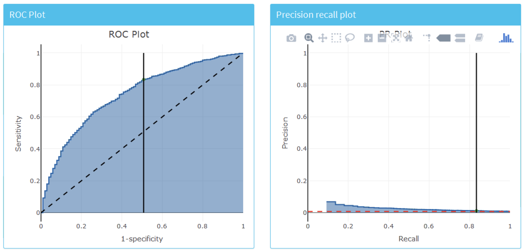
Figure 13.24: The ROC and precision-recall plots used to access the overall discrimination ability of the model.
Figure 13.25 shows the prediction and preference score distributions.
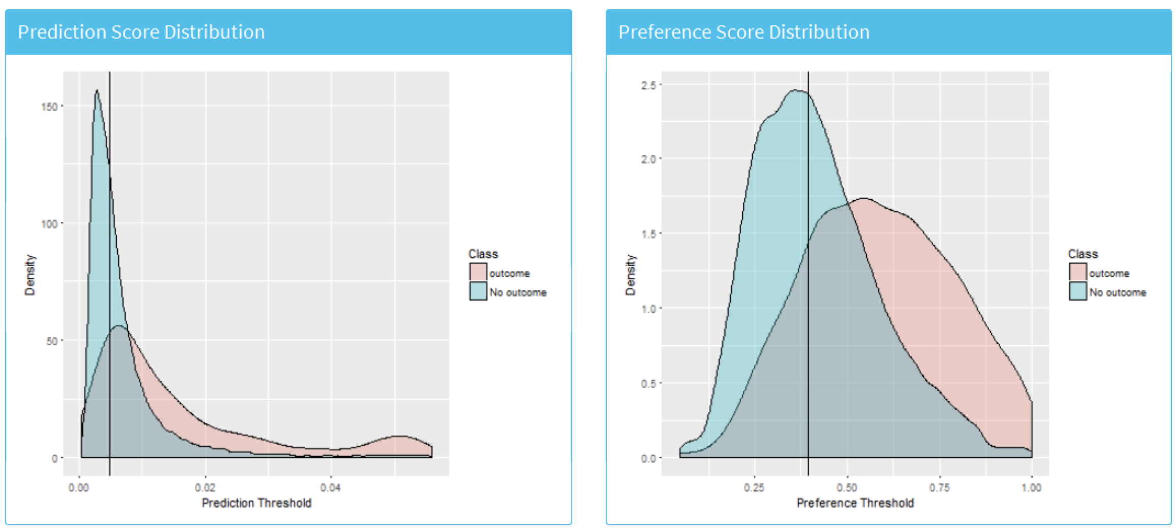
Figure 13.25: The predicted risk distribution for those with and without the outcome. The more these overlap the worse the discrimination
Finally, we can also inspect the calibration of the model by clicking on the “Calibration” tab. This displays the calibration plot and the demographic calibration shown in Figure 13.26.
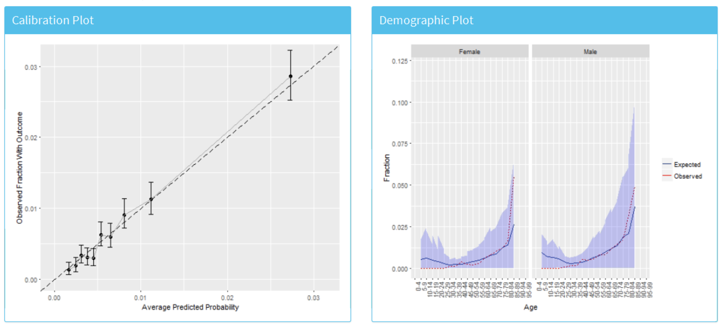
Figure 13.26: The risk stratified calibration and demographic calibration
We see that the average predicted risk appears to match the observed fraction who experienced the outcome within a year, so the model is well calibrated. Interestingly, the demographic calibration shows that the expected line is higher than the observed line for young patients, so we are predicting a higher risk for young age groups. Conversely, for the patients above 80 the model is predicting a lower risk than the observed risk. This may prompt us to develop separate models for the younger or older patients.
Viewing the Model
To inspect the final model, select the  option from the left hand menu. This will open a view containing plots for each variable in the model, shown in Figure 13.27, and a table summarizing all the candidate covariates, shown in Figure 13.28. The variable plots are separated into binary variables and continuous variables. The x-axis is the prevalence/mean in patients without the outcome and the y-axis is the prevalence/mean in patients with the outcome. Therefore, any variable’s dot falling above the diagonal is more common in patients with the outcome and any variable’s dot falling below the diagonal is less common in patients with the outcome.
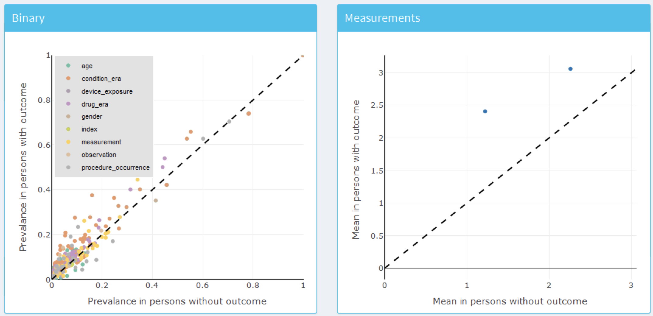
Figure 13.27: Model summary plots. Each dot corresponds to a variable included in the model.
The table in Figure 13.28 displays the name, value (coefficient if using a general linear model, or variable importance otherwise) for all the candidate covariates, outcome mean (the mean value for those who have the outcome) and non-outcome mean (the mean value for those who do not have the outcome).
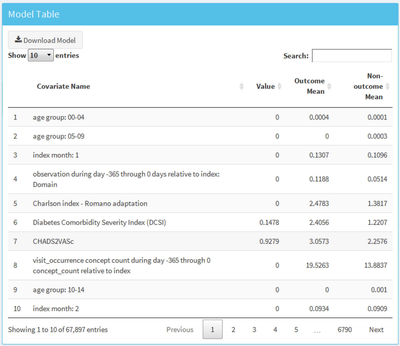
Figure 13.28: Model details table.
13.9 Additional Patient-Level Prediction Features
13.9.1 Journal Paper Generation
We have added functionality to automatically generate a word document we can use as start of a journal paper. It contains many of the generated study details and results. If we have performed external validation these results will can be added as well. Optionally, we can add a “Table 1” that contains data on many covariates for the target population. We can create the draft journal paper by running this function:
 createPlpJournalDocument(plpResult = <your plp results>,
             plpValidation = <your validation results>,
             plpData = <your plp data>,
             targetName = "<target population>",
             outcomeName = "<outcome>",
             table1 = F,
             connectionDetails = NULL,
             includeTrain = FALSE,
             includeTest = TRUE,
             includePredictionPicture = TRUE,
             includeAttritionPlot = TRUE,
             outputLocation = "<your location>")
For more details see the help page of the function.
13.10 Summary
Patient-level prediction aims to develop a model that predicts future events using data from the past.
The selection of the best machine algorithm for model development is an empirical question, i.e. it should be driven by the problem and data at hand.
The PatientLevelPrediction Package implements best practices for the development and validation of prediction models using data stored in the OMOP-CDM.
The dissemination of the model and its performance measures is implemented through interactive dashboards.
OHDSI’s prediction framework enables large-scale external validation of prediction models which is a pre-requisite for clinical adoption.
13.11 Exercises
Prerequisites
For these exercises we assume R, R-Studio and Java have been installed as described in Section 8.4.5. Also required are the SqlRender, DatabaseConnector, Eunomia and PatientLevelPrediction packages, which can be installed using:
install.packages(c("SqlRender", "DatabaseConnector", "remotes"))
remotes::install_github("ohdsi/Eunomia", ref = "v1.0.0")
remotes::install_github("ohdsi/PatientLevelPrediction")
The Eunomia package provides a simulated dataset in the CDM that will run inside your local R session. The connection details can be obtained using:
The CDM database schema is “main”. These exercises also make use of several cohorts. The createCohorts function in the Eunomia package will create these in the COHORT table:
Problem Definition
In patients that started using NSAIDs for the first time, predict who will develop a gastrointestinal (GI) bleed in the next year.
The NSAID new-user cohort has COHORT_DEFINITION_ID = 4. The GI bleed cohort has COHORT_DEFINITION_ID = 3.
Exercise 13.1 Using the PatientLevelPrediction R package, define the covariates you want to use for the prediction and extract the PLP data from the CDM. Create the summary of the PLP data.
Exercise 13.2 Revisit the design choices you have to make to define the final target population and specify these using the createStudyPopulation function. What will the effect of your choices be on the final size of the target population?
Exercise 13.3 Build a prediction model using LASSO and evaluate its performance using the Shiny application. How well is your model performing?
Suggested answers can be found in Appendix E.9.
References
Byrd, J. B., A. Adam, and N. J. Brown. 2006. “Angiotensin-converting enzyme inhibitor-associated angioedema.” Immunol Allergy Clin North Am 26 (4): 725–37.
Cicardi, M., L. C. Zingale, L. Bergamaschini, and A. Agostoni. 2004. “Angioedema associated with angiotensin-converting enzyme inhibitor use: outcome after switching to a different treatment.” Arch. Intern. Med. 164 (8): 910–13.
Norman, J. L., W. L. Holmes, W. A. Bell, and S. W. Finks. 2013. “Life-threatening ACE inhibitor-induced angioedema after eleven years on lisinopril.” J Pharm Pract 26 (4): 382–88.
O’Mara, N. B., and E. M. O’Mara. 1996. “Delayed onset of angioedema with angiotensin-converting enzyme inhibitors: case report and review of the literature.” Pharmacotherapy 16 (4): 675–79.
Reps, J. M., M. J. Schuemie, M. A. Suchard, P. B. Ryan, and P. R. Rijnbeek. 2018. “Design and implementation of a standardized framework to generate and evaluate patient-level prediction models using observational healthcare data.” Journal of the American Medical Informatics Association 25 (8): 969–75. https://doi.org/10.1093/jamia/ocy032.
Thompson, T., and M. A. Frable. 1993. “Drug-induced, life-threatening angioedema revisited.” Laryngoscope 103 (1 Pt 1): 10–12.